- Data Handling
- WHO Growth Standards
- Intergrowth Birth Standards
- Intergrowth Fetal Standards
- Growth Standard Vis
- Modeling
- get_fit
- fit_trajectory
- fit_all_trajectories
- get_fit_holdout_mse
- get_fit_holdout_errors
- plot.fittedTrajectory
- plot_z
- plot_velocity
- plot_zvelocity
- get_avail_methods
- fit_method.brokenstick
- fit_method.face
- fit_method.fda
- fit_method.gam
- fit_method.loess
- fit_method.lwmod
- fit_method.rlm
- fit_method.sitar
- fit_method.smooth.spline
- fit_method.wand
- auto_loess
- Summary Vis
- Multi-Study Vis
- Trelliscope Vis
- Divisions
- Data Sets
- Misc
- Unit Conversion
Healthy birth, growth & development
Authors: Ryan Hafen [aut, cre],Craig Anderson [ctb],Barret Schloerke [ctb]
Version: 0.3.6
License: MIT + file LICENSE
Description
A package for visual and analytical methods for the analysis of longitudinal growth data.
Depends
R (>= 3.1), datadr (>= 0.8.1), trelliscope (>= 0.9.2)
Imports
dplyr, lattice, rbokeh (>= 0.5.0), ggplot2, mgcv, MASS, numDeriv, gamlss.dist, fda, sitar (>= 1.0.3), DT, lme4, nlme, scales, crayon, stringdist
Suggests
testthat, packagedocs, brokenstick (>= 0.49), face (>= 0.1-2)
Data Handling
check_data
Check a dataset to ensure it will be compatible with hbgd methods
Usage
check_data(dat, has_height = TRUE, has_weight = TRUE, has_hcir = TRUE)Arguments
- dat
- a data frame
- has_height
- does this dataset contain anthropometric height data?
- has_weight
- does this dataset contain anthropometric weight data?
- has_hcir
- does this dataset contain anthropometric head circumference data?
Examples
check_data(cpp, has_hcir = FALSE)## Checking if data is a data frame...## [32m✓[39m## Checking variable name case...## [32m✓[39m## Checking for variable 'subjid'...## [32m✓[39m## Checking for variable 'agedays'...## [32m✓[39m## Checking for variable 'sex'...## [32m✓[39m## Checking values of variable 'sex'...## [32m✓[39m## Checking for variable 'lencm'...## [32m✓[39m## Checking for variable 'htcm'...## [32m✓[39m## Checking for variable 'wtkg'...## [32m✓[39m## Checking for both 'lencm' and 'htcm'...## Checking z-score variable 'haz' for height...## [32m✓[39m## Checking z-score variable 'waz' for weight...## [32m✓[39m## Checking to see if data is longitudinal...## [32m✓[39m## Checking names in data that are not standard 'hbgd' variables...## All checks passed!## As a final check, please ensure the units of measurement match## the variable descriptions (e.g. age in days, height in centimeters, etc.).smc <- brokenstick::smocc.hgtwgt
check_data(smc, has_hcir = FALSE)## Checking if data is a data frame...## [32m✓[39m## Checking variable name case...## [32m✓[39m## Checking for variable 'subjid'...## [31m✗[39m## Variable 'subjid' was not found in the data.## Closest matches (with index): id (2), bw (9)## Definition: Subject ID## This variable is required.## Please create or rename the appropriate variable.## To rename, choose the appropriate index i and:## names(dat)[i] <- 'subjid'## Checking for variable 'agedays'...## [31m✗[39m## Variable 'agedays' was not found in the data.## Closest matches (with index): age (5), ga (8)## Definition: Age since birth at examination (days)## This variable is required.## Please create or rename the appropriate variable.## To rename, choose the appropriate index i and:## names(dat)[i] <- 'agedays'## Checking for variable 'sex'...## [32m✓[39m## Checking values of variable 'sex'...## [31m✗[39m## All values of variable 'sex' must be 'Male' and 'Female'.## Checking for variable 'lencm'...## ## Variable 'lencm' was not found in the data.## Closest matches (with index): nrec (4), rec (3)## Definition: Recumbent length (cm)## This variable is not required but if it exists in the data## under a different name, please rename it to 'lencm'.## Checking for variable 'htcm'...## ## Variable 'htcm' was not found in the data.## Closest matches (with index): hgt (10), hgt.z (12)## Definition: Standing height (cm)## This variable is not required but if it exists in the data## under a different name, please rename it to 'htcm'.## Checking for variable 'wtkg'...## ## Variable 'wtkg' was not found in the data.## Closest matches (with index): wgt (11), hgt (10)## Definition: Weight (kg)## This variable is not required but if it exists in the data## under a different name, please rename it to 'wtkg'.## Checking for both 'lencm' and 'htcm'...## Checking names in data that are not standard 'hbgd' variables...## The following variables were found in the data:## src, id, rec, nrec, age, etn, ga, bw, hgt, wgt, hgt.z## Run view_variables() to see if any of these can be mapped## to an 'hbgd' variable name.## Some checks did not pass - please take action accordingly.names(smc)[2] <- "subjid"
names(smc)[5] <- "agedays"
smc$sex <- as.character(smc$sex)
smc$sex[smc$sex == "male"] <- "Male"
smc$sex[smc$sex == "female"] <- "Female"
names(smc)[10] <- "htcm"
names(smc)[11] <- "wtkg"
check_data(smc, has_hcir = FALSE)## Checking if data is a data frame...## [32m✓[39m## Checking variable name case...## [32m✓[39m## Checking for variable 'subjid'...## [32m✓[39m## Checking for variable 'agedays'...## [32m✓[39m## Checking for variable 'sex'...## [32m✓[39m## Checking values of variable 'sex'...## [32m✓[39m## Checking for variable 'lencm'...## ## Variable 'lencm' was not found in the data.## Closest matches (with index): nrec (4), rec (3)## Definition: Recumbent length (cm)## This variable is not required but if it exists in the data## under a different name, please rename it to 'lencm'.## Checking for variable 'htcm'...## [32m✓[39m## Checking for variable 'wtkg'...## [32m✓[39m## Checking for both 'lencm' and 'htcm'...## Checking z-score variable 'haz' for height...## ## Could not find height z-score variable 'haz'.## If it exists, rename it to 'haz'.## If it doesn't exist, create it with:## dat$haz <- who_htcm2zscore(dat$agedays, dat$htcm, dat$sex)## Checking z-score variable 'waz' for weight...## ## Could not find weight z-score variable 'waz'.## If it exists, rename it to 'waz'.## If it doesn't exist, create it with:## dat$waz <- who_wtkg2zscore(dat$agedays, dat$wtkg, dat$sex)## Checking to see if data is longitudinal...## [32m✓[39m## Checking names in data that are not standard 'hbgd' variables...## The following variables were found in the data:## src, rec, nrec, etn, ga, bw, hgt.z## Run view_variables() to see if any of these can be mapped## to an 'hbgd' variable name.## All checks passed!## As a final check, please ensure the units of measurement match## the variable descriptions (e.g. age in days, height in centimeters, etc.).names(smc)[12] <- "haz"
smc$waz <- who_wtkg2zscore(smc$agedays, smc$wtkg, smc$sex)
smc$agedays <- smc$agedays * 365.25
check_data(smc, has_hcir = FALSE)## Checking if data is a data frame...## [32m✓[39m## Checking variable name case...## [32m✓[39m## Checking for variable 'subjid'...## [32m✓[39m## Checking for variable 'agedays'...## [32m✓[39m## Checking for variable 'sex'...## [32m✓[39m## Checking values of variable 'sex'...## [32m✓[39m## Checking for variable 'lencm'...## ## Variable 'lencm' was not found in the data.## Closest matches (with index): nrec (4), rec (3)## Definition: Recumbent length (cm)## This variable is not required but if it exists in the data## under a different name, please rename it to 'lencm'.## Checking for variable 'htcm'...## [32m✓[39m## Checking for variable 'wtkg'...## [32m✓[39m## Checking for both 'lencm' and 'htcm'...## Checking z-score variable 'haz' for height...## [32m✓[39m## Checking z-score variable 'waz' for weight...## [32m✓[39m## Checking to see if data is longitudinal...## [32m✓[39m## Checking names in data that are not standard 'hbgd' variables...## The following variables were found in the data:## src, rec, nrec, etn, ga, bw## Run view_variables() to see if any of these can be mapped## to an 'hbgd' variable name.## All checks passed!## As a final check, please ensure the units of measurement match## the variable descriptions (e.g. age in days, height in centimeters, etc.).Get subject and time data
Get subject-level or time-varying variables and rows of longitudinal data
Usage
get_subject_data(dat)
get_time_data(dat)
Arguments
- dat
- data frame with longitudinal data
fix_height
Merge ‘htcm’ and ‘lencm’ into the ‘htcm’ variable
Usage
fix_height(dat)Arguments
- dat
- data
add_holdout_ind
Add indicator column for per-subject holdout
Usage
add_holdout_ind(dat, random = TRUE)Arguments
- dat
- data
- random
- if TRUE, a random observation per subject will be designated as the holdout, if FALSE, the endpoint for each subject will be designated as the holdout
get_data_attributes
Infer and attach attributes to a longitudinal growth study dataset
Infer attributes such as variable types of a longitudinal growth study and add as attributes to the dataset.
Usage
get_data_attributes(dat, meta = NULL, study_meta = NULL)Arguments
- dat
- a longitudinal growth study dataset
- meta
- a data frame of meta data about the variables (a row for each variable)
- study_meta
- a single-row data frame or named list of meta data about the study (such as study description, etc.)
Details
attributes added: - subjectlevel_vars: vector of names of subject-level variables - timevarying_vars: vector of names of time-varying variables - time_vars: vector of names of measures of age - var_summ: data frame containing variable summaries with columns variable, label, type[subject id, time indicator, time-varying, constant], n_unique - subj_count: data frame of counts of records for each subject with columns subjid, n - n_subj: scalar containing total number of subjects - labels named list of variable labels - either populated by matching names with a pre-set list of labels (see hbgd_labels) or from a list provided from the meta argument - study_meta: data frame of meta data (if provided from the study_meta argument) - short_id: scalar containing the short unique identifier for the study (if study_meta is provided)
Examples
cpp <- get_data_attributes(cpp)
str(attributes(cpp))
## List of 4
## $ names : chr [1:37] "subjid" "agedays" "wtkg" "htcm" ...
## $ row.names: int [1:1912] 1 2 3 4 5 6 7 8 9 10 ...
## $ hbgd :List of 8
## ..$ labels :List of 37
## .. ..$ subjid : chr "Subject ID"
## .. ..$ agedays : chr "Age since birth at examination (days)"
## .. ..$ wtkg : chr "Weight (kg)"
## .. ..$ htcm : chr "Standing height (cm)"
## .. ..$ lencm : chr "Recumbent length (cm)"
## .. ..$ bmi : chr "BMI (kg/m**2)"
## .. ..$ waz : chr "Weight for age z-score"
## .. ..$ haz : chr "Length/height for age z-score"
## .. ..$ whz : chr "Weight for length/height z-score"
## .. ..$ baz : chr "BMI for age z-score"
## .. ..$ siteid : chr "Investigational Site ID"
## .. ..$ sexn : chr "Sex (numeric)"
## .. ..$ sex : chr "Sex"
## .. ..$ feedingn: chr "Feeding practice (numeric)"
## .. ..$ feeding : chr "Feeding practice"
## .. ..$ gagebrth: chr "Gestational age at birth (days)"
## .. ..$ birthwt : chr "Birth weight (gm)"
## .. ..$ birthlen: chr "Birth length (cm)"
## .. ..$ apgar1 : chr "APGAR Score 1 min after birth"
## .. ..$ apgar5 : chr "APGAR Score 5 min after birth"
## .. ..$ mage : chr "Maternal age at birth of child (yrs)"
## .. ..$ mracen : chr "Maternal race (num)"
## .. ..$ mrace : chr "Maternal race"
## .. ..$ mmaritn : chr "Mothers marital status (num)"
## .. ..$ mmarit : chr "Mothers marital status"
## .. ..$ meducyrs: chr "Mother, years of education"
## .. ..$ sesn : chr "Socioeconomic status of parent (num)"
## .. ..$ ses : chr "Socioeconomic status of parent"
## .. ..$ parity : chr "Maternal parity"
## .. ..$ gravida : chr "Maternal num pregnancies"
## .. ..$ smoked : chr "Mom smoked during pregnancy?"
## .. ..$ mcignum : chr "Num cigarettes mom smoked per day"
## .. ..$ preeclmp: chr "Preeclampsia"
## .. ..$ comprisk: chr "Pregnancy complications/risk factors"
## .. ..$ geniq : chr "Intelligence Quotient General Intelligence IQ"
## .. ..$ sysbp : chr "Systolic Blood Pressure"
## .. ..$ diabp : chr "Diastolic Blood Pressure"
## ..$ subjectlevel_vars: chr [1:24] "siteid" "sexn" "sex" "feedingn" ...
## ..$ timevarying_vars : chr [1:11] "wtkg" "htcm" "lencm" "bmi" ...
## ..$ time_vars : chr "agedays"
## ..$ var_summ :Classes 'var_summ' and 'data.frame': 37 obs. of 5 variables:
## .. ..$ variable: chr [1:37] "subjid" "agedays" "wtkg" "htcm" ...
## .. ..$ label : chr [1:37] "Subject ID" "Age since birth at examination (days)" "Weight (kg)" "Standing height (cm)" ...
## .. ..$ type : chr [1:37] "subject id" "time indicator" "time-varying" "time-varying" ...
## .. ..$ vtype : chr [1:37] "num" "cat" "num" "num" ...
## .. ..$ n_unique: int [1:37] 500 5 417 81 42 956 527 137 413 392 ...
## ..$ subj_count :'data.frame': 500 obs. of 2 variables:
## .. ..$ subjid: int [1:500] 1 2 3 4 5 6 7 8 9 10 ...
## .. ..$ n : int [1:500] 3 4 1 1 1 1 4 5 5 2 ...
## ..$ n_subj : int 500
## ..$ ad_tab :Classes 'ad_tab' and 'data.frame': 5 obs. of 2 variables:
## .. ..$ agedays: int [1:5] 1 123 366 1462 2558
## .. ..$ n : int [1:5] 500 460 428 137 387
## $ class : chr "data.frame"See also
WHO Growth Standards
generic centile/z-score to value
Convert WHO z-scores/centiles to anthro measurements (generic)
Get values of a specified measurement for a given WHO centile/z-score and growth standard pair (e.g. length vs. age) and sex over a specified grid
Usage
who_centile2value(x, p = 50, x_var = "agedays", y_var = "htcm", sex = "Female", data = NULL)
who_zscore2value(x, z = 0, y_var = "htcm", x_var = "agedays", sex = "Female", data = NULL)
Arguments
- x
- vector specifying the values of x over which to provide the centiles for y
- p
- centile or vector of centiles at which to compute values (a number between 0 and 100 - 50 is median)
- x_var
- x variable name (typically “agedays”) - see details
- y_var
- y variable name (typically “htcm” or “wtkg”) that specifies which variable of values should be returned for the specified value of q - see details
- sex
- “Male” or “Female”
- data
- optional data frame that supplies any of the other variables provided to the function
- z
- z-score or vector of z-scores at which to compute values
Details
for all supported pairings of x_var and y_var, type names(who)
Examples
# median height vs. age for females
x <- seq(0, 365, by = 7)
med <- who_centile2value(x)
plot(x, med, xlab = "age in days", ylab = "median female height (cm)")
# 99th percentile of weight vs. age for males from age 0 to 1461 days
dat <- data.frame(x = rep(seq(0, 1461, length = 100), 2),
  sex = rep(c("Male", "Female"), each = 100))
dat$p99 <- who_centile2value(x, p = 99, y_var = "wtkg", sex = sex, data = dat)
lattice::xyplot(kg2lb(p99) ~ days2years(x), groups = sex, data = dat,
  ylab = "99th percentile weight (pounds) for males",
  xlab = "age (years)", auto.key = TRUE)
See also
generic value to centile/z-score
Convert anthro measurements to WHO z-scores/centiles (generic)
Compute z-scores or centiles with respect to the WHO growth standard for given values of x vs. y (typically x is “agedays” and y is a measure like “htcm”).
Usage
who_value2zscore(x, y, x_var = "agedays", y_var = "htcm", sex = "Female", data = NULL)
who_value2centile(x, y, x_var = "agedays", y_var = "htcm", sex = "Female", data = NULL)
Arguments
- x
-
value or vector of values that correspond to a measure defined by
x_var - y
-
value or vector of values that correspond to a measure defined by
y_var - x_var
- x variable name (typically “agedays”) - see details
- y_var
- y variable name (typically “htcm” or “wtkg”) - see details
- sex
- “Male” or “Female”
- data
- optional data frame that supplies any of the other variables provided to the function
Details
for all supported pairings of x_var and y_var, type names(who)
Examples
# z-scores
who_value2zscore(1670, in2cm(44))
## [1] 1.117365who_value2zscore(1670, lb2kg(48), y_var = "wtkg")## [1] 1.527048who_value2centile(1670, in2cm(44))## [1] 86.80809who_value2centile(1670, lb2kg(48), y_var = "wtkg")## [1] 93.66255# add haz derived from WHO data and compare to that provided with data
cpp$haz2 <- who_value2zscore(x = agedays, y = lencm, sex = sex, data = cpp)
plot(cpp$haz, cpp$haz2)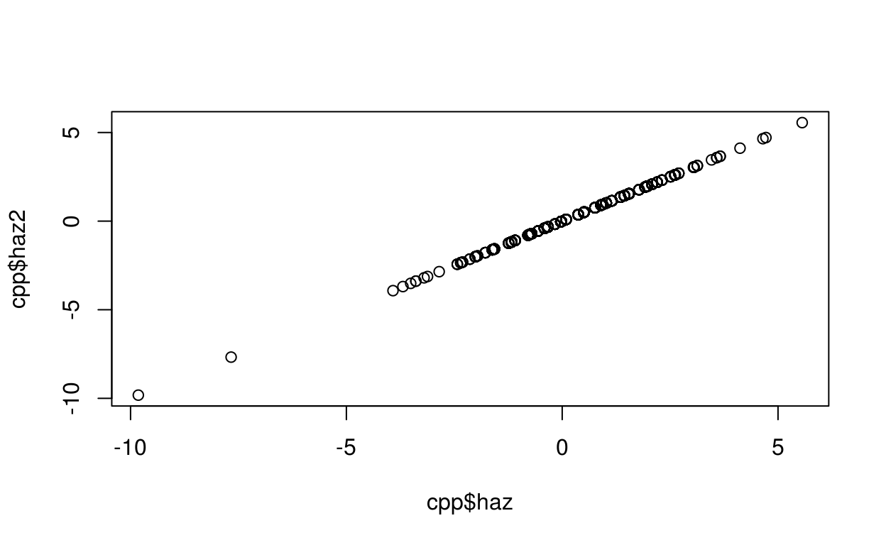
# note that you can also do it this way
#' cpp$haz2 <- who_value2zscore(cpp$agedays, cpp$lencm, sex = cpp$sex)
See also
specific centile/z-score to value
Convert WHO z-scores/centiles to anthro measurements
Usage
who_zscore2htcm(agedays, z = 0, sex = "Female")
who_zscore2wtkg(agedays, z = 0, sex = "Female")
who_zscore2bmi(agedays, z = 0, sex = "Female")
who_zscore2hcircm(agedays, z = 0, sex = "Female")
who_zscore2muaccm(agedays, z = 0, sex = "Female")
who_zscore2ssftmm(agedays, z = 0, sex = "Female")
who_zscore2tsftmm(agedays, z = 0, sex = "Female")
who_centile2htcm(agedays, p = 50, sex = "Female")
who_centile2wtkg(agedays, p = 50, sex = "Female")
who_centile2bmi(agedays, p = 50, sex = "Female")
who_centile2hcircm(agedays, p = 50, sex = "Female")
who_centile2muaccm(agedays, p = 50, sex = "Female")
who_centile2ssftmm(agedays, p = 50, sex = "Female")
who_centile2tsftmm(agedays, p = 50, sex = "Female")
Arguments
- agedays
- age in days
- z
- z-score(s) to convert
- sex
- “Male” or “Female”
- p
- centile(s) to convert (must be between 0 and 100)
Examples
htcm <- who_zscore2htcm(cpp$agedays, cpp$haz, cpp$sex)specific value to centile/z-score
Convert anthro measurements to WHO z-scores/centiles
Usage
who_wtkg2zscore(agedays, wtkg, sex = "Female")
who_htcm2zscore(agedays, htcm, sex = "Female")
who_bmi2zscore(agedays, bmi, sex = "Female")
who_hcircm2zscore(agedays, hcircm, sex = "Female")
who_muaccm2zscore(agedays, muaccm, sex = "Female")
who_ssftmm2zscore(agedays, ssftmm, sex = "Female")
who_tsftmm2zscore(agedays, tsftmm, sex = "Female")
who_wtkg2centile(agedays, wtkg, sex = "Female")
who_htcm2centile(agedays, htcm, sex = "Female")
who_bmi2centile(agedays, bmi, sex = "Female")
who_hcircm2centile(agedays, hcircm, sex = "Female")
who_muaccm2centile(agedays, muaccm, sex = "Female")
who_ssftmm2centile(agedays, ssftmm, sex = "Female")
who_tsftmm2centile(agedays, tsftmm, sex = "Female")
Arguments
- agedays
- age in days
- wtkg
- weight (kg) measurement(s) to convert
- sex
- “Male” or “Female”
- htcm
- height(cm) measurement(s) to convert
- bmi
- body-mass index measurement(s) to convert
- hcircm
- head circumference (cm) measurement(s) to convert
- muaccm
- mid-upper arm circumference (cm) measurement(s) to convert
- ssftmm
- subscalpular skinfold (mm) measurement(s) to convert
- tsftmm
- triceps skinfold (mm) measurement(s) to convert
Examples
haz <- who_htcm2zscore(cpp$agedays, cpp$htcm, cpp$sex)Intergrowth Birth Standards
generic centile/z-score to value
Convert birth measurements to INTERGROWTH z-scores/centiles (generic)
Usage
igb_centile2value(gagebrth, p = 50, var = "lencm", sex = "Female")
igb_zscore2value(gagebrth, z = 0, var = "lencm", sex = "Female")
Arguments
- gagebrth
- gestational age at birth in days
- p
- centile(s) to convert (must be between 0 and 100)
- var
- the name of the measurement to convert (“lencm”, “wtkg”, “hcircm”)
- sex
- “Male” or “Female”
- z
- z-score(s) to convert
Note
For gestational ages between 24 and 33 weeks, the INTERGROWTH very early preterm standard is used.
References
International standards for newborn weight, length, and head circumference by gestational age and sex: the Newborn Cross-Sectional Study of the INTERGROWTH-21st Project Villar, José et al. The Lancet, Volume 384, Issue 9946, 857-868
INTERGROWTH-21st very preterm size at birth reference charts. Lancet 2016 doi.org/10.1016/S0140-6736(16) 00384-6. Villar, José et al.
Examples
# get 99th centile for Male birth weights across some gestational ages
igb_centile2value(232:300, 99, var = "wtkg", sex = "Male")
## [1] 3.095594 3.134276 3.172468 3.210176 3.247402 3.284150 3.320425
## [8] 3.356229 3.391566 3.426440 3.460857 3.494817 3.528324 3.561383
## [15] 3.593996 3.626168 3.657900 3.689198 3.720065 3.750502 3.780513
## [22] 3.810103 3.839274 3.868027 3.896370 3.924301 3.951826 3.978946
## [29] 4.005666 4.031988 4.057915 4.083450 4.108594 4.133353 4.157728
## [36] 4.181721 4.205336 4.228576 4.251442 4.273939 4.296067 4.317829
## [43] 4.339230 4.360270 4.380952 4.401281 4.421255 4.440879 4.460156
## [50] 4.479087 4.497674 4.515922 4.533831 4.551403 4.568641 4.585547
## [57] 4.602125 4.618375 4.634299 4.649901 4.665183 4.680145 4.694791
## [64] 4.709122 4.723141 4.736849 4.750250 4.763343 4.776132generic value to centile/z-score
Convert birth measurements to INTERGROWTH z-scores/centiles (generic)
Usage
igb_value2centile(gagebrth, val, var = "lencm", sex = "Female")
igb_value2zscore(gagebrth, val, var = "lencm", sex = "Female")
Arguments
- gagebrth
- gestational age at birth in days
- val
- the value(s) of the anthro measurement to convert
- var
- the name of the measurement to convert (“lencm”, “wtkg”, “hcircm”)
- sex
- “Male” or “Female”
Note
For gestational ages between 24 and 33 weeks, the INTERGROWTH very early preterm standard is used.
References
International standards for newborn weight, length, and head circumference by gestational age and sex: the Newborn Cross-Sectional Study of the INTERGROWTH-21st Project Villar, José et al. The Lancet, Volume 384, Issue 9946, 857-868
INTERGROWTH-21st very preterm size at birth reference charts. Lancet 2016 doi.org/10.1016/S0140-6736(16) 00384-6. Villar, José et al.
Examples
# get Male birth length z-scores
# first we need just 1 record per subject with subject-level data
cppsubj <- get_subject_data(cpp)
cppsubj <- subset(cppsubj, sex == "Male")
igb_value2zscore(cpp$gagebrth, cpp$birthlen, var = "lencm", sex = "Male")
## [1] 2.57008863 2.57008863 2.57008863 0.66769390 0.66769390
## [6] 0.66769390 0.66769390 2.77551410 0.24012569 1.20761609
## [11] 0.43007110 1.53920598 1.53920598 1.53920598 1.53920598
## [16] 1.53920598 1.53920598 1.53920598 1.53920598 1.53920598
## [21] 2.57008863 2.57008863 2.57008863 2.57008863 2.57008863
## [26] NA NA 1.37080474 1.37080474 1.37080474
## [31] 2.08629993 2.08629993 2.08167545 2.08167545 2.08167545
## [36] -0.92887191 -0.92887191 -0.92887191 -0.92887191 -0.17659363
## [41] -0.17659363 -0.17659363 -0.17659363 -0.17659363 0.43007110
## [46] 0.43007110 0.43007110 0.43007110 0.04777744 0.04777744
## [51] 0.04777744 0.04777744 -0.95427104 -0.95427104 -0.95427104
## [56] -0.95427104 -0.95427104 0.04777744 0.04777744 0.04777744
## [61] 0.04777744 0.10144540 0.10144540 0.10144540 1.01947447
## [66] 1.01947447 1.01947447 1.01947447 1.26177582 1.26177582
## [71] 1.26177582 1.26177582 1.26177582 1.01947447 1.01947447
## [76] 1.01947447 1.01947447 1.01947447 0.04777744 0.04777744
## [81] 0.04777744 0.04777744 0.04777744 2.08629993 2.08629993
## [86] 2.08629993 2.08629993 0.43007110 0.43007110 0.43007110
## [91] 0.43007110 0.04777744 2.08629993 2.08629993 2.08629993
## [96] 0.81893628 0.81893628 0.81893628 1.01947447 1.01947447
## [101] 1.01947447 1.01947447 0.24012569 0.24012569 0.24012569
## [106] 0.24012569 0.94776774 0.94776774 0.94776774 0.94776774
## [111] 1.26326658 1.26326658 1.26326658 1.26326658 1.26326658
## [116] 0.04777744 0.04777744 0.04777744 0.04777744 0.66769390
## [121] 0.66769390 0.66769390 -0.17659363 -0.17659363 -0.17659363
## [126] -0.17659363 0.43007110 0.43007110 0.43007110 0.43007110
## [131] 1.57506493 1.57506493 1.57506493 1.57506493 -0.57693404
## [136] -0.57693404 -0.57693404 -0.57693404 -1.18192366 -1.18192366
## [141] -1.18192366 -1.18192366 -1.18192366 0.32057449 0.32057449
## [146] 0.32057449 0.32057449 -0.32198638 -0.32198638 -0.32198638
## [151] -0.32198638 -0.32198638 NA NA NA
## [156] 1.01947447 1.01947447 1.01947447 -0.32198638 -0.32198638
## [161] -0.32198638 -0.32198638 0.32057449 0.32057449 0.32057449
## [166] 0.43007110 0.43007110 0.43007110 1.84381500 1.84381500
## [171] 1.84381500 0.24012569 0.24012569 0.24012569 0.24012569
## [176] 1.88394745 1.88394745 1.88394745 1.88394745 1.88394745
## [181] -0.95427104 -0.95427104 -0.95427104 -0.95427104 -0.95427104
## [186] -0.32198638 -0.32198638 -0.32198638 -0.32198638 -0.32198638
## [191] 1.57506493 1.57506493 1.57506493 1.57506493 -0.57693404
## [196] -0.57693404 -0.57693404 -0.57693404 0.04777744 0.04777744
## [201] -1.88881195 -1.88881195 -1.88881195 -1.88881195 0.43007110
## [206] 0.43007110 0.43007110 -0.57693404 -0.57693404 -0.57693404
## [211] -0.57693404 0.10144540 0.10144540 0.10144540 2.54912777
## [216] 2.54912777 2.54912777 2.54912777 1.53920598 1.53920598
## [221] 1.53920598 1.53920598 -0.01724797 -0.01724797 -0.01724797
## [226] -0.01724797 -0.17659363 -0.17659363 -0.17659363 -0.17659363
## [231] 0.04777744 0.04777744 0.04777744 0.04777744 0.04777744
## [236] 2.31733522 2.31733522 2.31733522 2.31733522 2.31733522
## [241] 2.31733522 0.32057449 0.32057449 0.32057449 0.32057449
## [246] 0.32057449 0.32057449 1.53920598 1.53920598 1.53920598
## [251] 2.54912777 2.54912777 2.54912777 2.54912777 -1.02459617
## [256] -1.02459617 -1.02459617 -2.82067962 0.63678619 0.63678619
## [261] 0.63678619 0.63678619 0.66769390 0.66769390 0.66769390
## [266] 0.66769390 1.37080474 1.37080474 1.37080474 1.37080474
## [271] 0.24012569 0.24012569 0.24012569 0.24012569 3.15541741
## [276] 3.15541741 3.15541741 3.15541741 0.32057449 0.32057449
## [281] 0.32057449 0.32057449 -0.57693404 -0.57693404 -0.57693404
## [286] -0.57693404 0.24012569 0.24012569 0.24012569 0.24012569
## [291] 2.31733522 2.31733522 2.31733522 2.31733522 2.08167545
## [296] 2.08167545 2.08167545 2.08167545 1.53920598 1.53920598
## [301] 1.53920598 1.53920598 0.66769390 0.66769390 0.66769390
## [306] 0.66769390 0.66769390 1.81440917 1.81440917 1.81440917
## [311] 1.81440917 1.57506493 1.57506493 1.57506493 1.57506493
## [316] 1.26177582 1.26177582 1.26177582 1.26177582 1.26177582
## [321] 1.26177582 1.26177582 1.81440917 1.81440917 1.81440917
## [326] 1.81440917 1.81440917 1.26326658 1.26326658 1.26326658
## [331] 1.26326658 NA NA NA NA
## [336] -0.32198638 -0.32198638 -0.32198638 -0.32198638 2.35247762
## [341] 2.35247762 2.35247762 2.35247762 2.35247762 2.35247762
## [346] 2.35247762 2.35247762 2.35247762 2.08629993 2.08629993
## [351] 2.08629993 2.08629993 2.76890374 2.76890374 2.76890374
## [356] 2.76890374 2.08629993 2.08629993 2.08629993 2.08629993
## [361] 2.31733522 2.31733522 2.31733522 2.31733522 0.32057449
## [366] 0.32057449 0.32057449 0.32057449 0.04777744 -0.57693404
## [371] -0.57693404 1.26177582 1.26177582 1.26177582 1.26177582
## [376] -1.18192366 -1.18192366 -1.18192366 -1.18192366 0.94776774
## [381] 0.94776774 0.94776774 0.94776774 -0.95427104 -0.95427104
## [386] -0.95427104 -0.95427104 0.66523053 0.66523053 0.66523053
## [391] 0.66523053 0.66523053 -0.57693404 -0.57693404 -0.57693404
## [396] -0.57693404 -0.57693404 -0.17659363 -0.17659363 -0.17659363
## [401] -0.17659363 -0.34918388 -0.34918388 -0.34918388 -0.34918388
## [406] 2.31733522 2.31733522 2.31733522 -0.32198638 -0.32198638
## [411] -0.32198638 -0.32198638 0.04777744 0.04777744 0.04777744
## [416] 0.04777744 1.81440917 1.81440917 1.81440917 1.81440917
## [421] 0.94776774 0.94776774 0.94776774 0.94776774 0.43007110
## [426] 0.43007110 0.43007110 0.43007110 1.53920598 1.53920598
## [431] 1.53920598 1.53920598 1.53920598 NA NA
## [436] NA NA -0.57693404 -0.57693404 -0.57693404
## [441] -0.57693404 -0.77955940 -0.77955940 -0.77955940 -0.77955940
## [446] -0.77955940 0.24012569 0.24012569 0.24012569 0.24012569
## [451] 0.94776774 0.94776774 0.94776774 0.94776774 2.57008863
## [456] 2.57008863 2.57008863 2.57008863 2.57008863 1.01947447
## [461] 1.01947447 1.01947447 1.84381500 1.84381500 1.84381500
## [466] 1.57506493 1.57506493 1.57506493 1.57506493 -5.80376219
## [471] -5.80376219 -5.80376219 -5.80376219 2.76890374 2.76890374
## [476] 2.76890374 2.76890374 2.76890374 -0.77955940 -0.77955940
## [481] -0.77955940 -0.77955940 0.94776774 0.94776774 0.94776774
## [486] 0.94776774 1.53920598 1.53920598 1.53920598 1.53920598
## [491] 1.53920598 1.53920598 1.53920598 1.53920598 1.53920598
## [496] 1.53920598 -0.57693404 -0.57693404 -0.57693404 -0.57693404
## [501] 0.04777744 0.04777744 0.04777744 0.66769390 0.66769390
## [506] 0.66769390 0.66769390 0.66769390 1.37080474 1.37080474
## [511] 1.37080474 1.37080474 0.32057449 0.32057449 0.32057449
## [516] 0.32057449 0.66769390 0.66769390 0.66769390 0.66769390
## [521] 0.66769390 -1.18192366 -1.18192366 -1.18192366 -1.18192366
## [526] -5.39174617 -5.39174617 -5.39174617 -5.39174617 -5.39174617
## [531] -0.32198638 -0.32198638 -0.32198638 -2.10044386 -2.10044386
## [536] -2.10044386 1.81440917 1.81440917 1.81440917 1.81440917
## [541] 0.10144540 0.10144540 0.10144540 0.10144540 0.10144540
## [546] 2.31733522 2.31733522 2.31733522 2.31733522 0.04777744
## [551] 0.04777744 0.04777744 0.04777744 0.04777744 NA
## [556] NA NA NA 0.66769390 0.66769390
## [561] 0.66769390 0.32057449 0.32057449 0.32057449 1.26177582
## [566] 1.26177582 1.26177582 1.26177582 -0.32198638 -0.32198638
## [571] -0.32198638 -0.32198638 0.04777744 0.04777744 0.04777744
## [576] 0.04777744 NA -1.55221271 -1.55221271 -0.57693404
## [581] -0.57693404 -0.57693404 -0.57693404 0.94776774 -4.28567708
## [586] -4.28567708 -4.28567708 -4.28567708 -3.21277379 -3.21277379
## [591] -3.21277379 -3.21277379 -3.21277379 -1.74780621 -1.74780621
## [596] -1.74780621 -1.74780621 -0.67380818 -0.67380818 -0.67380818
## [601] -0.67380818 2.31733522 2.31733522 2.31733522 0.04777744
## [606] 0.04777744 0.04777744 0.04777744 -1.48019642 -1.48019642
## [611] -1.48019642 -1.48019642 1.26177582 1.26177582 1.26177582
## [616] 1.26177582 -0.95427104 -0.95427104 -0.95427104 0.32057449
## [621] 0.32057449 0.32057449 1.81440917 1.81440917 1.81440917
## [626] -1.74780621 -1.74780621 -1.74780621 NA 0.43007110
## [631] 0.43007110 0.43007110 0.43007110 -0.77955940 -0.77955940
## [636] -0.77955940 -0.77955940 -0.77955940 1.20761609 1.20761609
## [641] 1.20761609 1.20761609 1.20761609 -0.34918388 -0.34918388
## [646] -0.34918388 -0.34918388 0.81893628 0.81893628 0.81893628
## [651] 0.81893628 0.81893628 1.20761609 1.20761609 1.20761609
## [656] 1.20761609 1.20761609 1.26177582 1.26177582 1.26177582
## [661] -0.77955940 -0.77955940 -0.77955940 -0.77955940 1.01947447
## [666] 1.01947447 1.01947447 1.01947447 2.08167545 2.08167545
## [671] 2.08167545 2.08167545 1.84381500 1.84381500 1.84381500
## [676] 1.84381500 0.94776774 0.94776774 0.94776774 0.94776774
## [681] 2.76890374 2.76890374 0.04777744 1.81440917 1.81440917
## [686] 1.81440917 1.81440917 1.81440917 1.53920598 1.53920598
## [691] 1.53920598 1.53920598 -0.67380818 -0.67380818 -0.67380818
## [696] -0.67380818 0.04777744 0.04777744 0.04777744 0.94776774
## [701] 0.94776774 0.94776774 2.35247762 2.35247762 2.35247762
## [706] 2.35247762 -0.17659363 -0.17659363 -0.17659363 -0.17659363
## [711] 0.66769390 0.66769390 0.66769390 0.66769390 0.66769390
## [716] 2.08167545 2.08167545 2.08167545 2.08167545 0.32057449
## [721] 0.32057449 0.32057449 0.32057449 0.32057449 0.43007110
## [726] 0.43007110 0.43007110 0.43007110 NA NA
## [731] NA NA NA 2.76890374 2.76890374
## [736] 0.43007110 0.43007110 0.43007110 0.43007110 0.32057449
## [741] 0.32057449 0.32057449 0.32057449 -0.95427104 -0.95427104
## [746] -0.95427104 -0.95427104 -1.74780621 -1.74780621 -1.74780621
## [751] -1.74780621 0.66769390 0.66769390 0.66769390 0.66769390
## [756] 0.66769390 -1.35698291 -1.35698291 -1.35698291 -1.35698291
## [761] -1.35698291 NA NA NA NA
## [766] 2.54912777 2.54912777 2.54912777 2.54912777 2.54912777
## [771] NA -1.30459500 -1.30459500 -1.30459500 -1.30459500
## [776] 2.76890374 2.76890374 2.76890374 2.76890374 NA
## [781] NA NA NA NA 0.32057449
## [786] 0.32057449 0.32057449 0.32057449 0.32057449 1.53920598
## [791] 1.53920598 1.53920598 1.53920598 1.01947447 1.01947447
## [796] 1.01947447 1.01947447 1.01947447 2.96436156 2.96436156
## [801] 2.96436156 2.96436156 2.96436156 2.18498566 2.18498566
## [806] 2.18498566 0.66769390 0.66769390 0.66769390 0.66769390
## [811] 3.39217340 3.39217340 3.39217340 3.39217340 NA
## [816] NA NA NA 3.49617450 3.49617450
## [821] 3.49617450 3.49617450 3.49617450 1.26177582 1.26177582
## [826] 1.26177582 1.26177582 3.53071911 3.53071911 3.53071911
## [831] 3.53071911 3.53071911 1.71653479 1.71653479 1.71653479
## [836] 1.71653479 1.71653479 0.81893628 0.81893628 0.81893628
## [841] 0.81893628 0.81893628 3.33560617 3.33560617 3.33560617
## [846] 3.33560617 3.33560617 2.18498566 2.18498566 2.18498566
## [851] 2.18498566 -0.95427104 -0.95427104 -0.95427104 -0.95427104
## [856] 0.04777744 0.04777744 0.04777744 0.04777744 0.04777744
## [861] -2.10044386 -2.10044386 -2.10044386 0.66769390 0.66769390
## [866] 0.66769390 0.66769390 2.61075974 2.61075974 2.61075974
## [871] 2.61075974 2.61075974 0.24012569 0.24012569 0.24012569
## [876] 0.24012569 0.24012569 -0.17659363 -0.17659363 -0.17659363
## [881] -0.17659363 0.43007110 0.43007110 0.43007110 0.66769390
## [886] 0.66769390 0.66769390 0.66769390 0.04777744 0.04777744
## [891] 0.04777744 1.81440917 1.81440917 1.81440917 -1.18192366
## [896] -1.18192366 -1.18192366 -1.18192366 -0.17659363 -0.17659363
## [901] -0.17659363 -0.17659363 -0.17659363 2.35247762 2.35247762
## [906] 2.35247762 2.35247762 NA NA NA
## [911] NA NA -2.59359762 -2.59359762 -2.59359762
## [916] -2.59359762 -1.30459500 -1.30459500 -1.30459500 1.81440917
## [921] 1.81440917 1.81440917 1.81440917 1.81440917 0.66769390
## [926] 0.66769390 0.66769390 0.66769390 NA NA
## [931] NA NA 2.31733522 2.31733522 2.31733522
## [936] 2.31733522 1.57506493 1.57506493 1.57506493 1.57506493
## [941] 1.26177582 1.26177582 1.26177582 1.26177582 1.26177582
## [946] 2.08629993 2.08629993 2.08629993 0.43007110 0.43007110
## [951] 0.43007110 0.43007110 0.43007110 0.43007110 0.43007110
## [956] 0.43007110 -2.26398780 -2.26398780 -2.26398780 0.43007110
## [961] 0.43007110 0.43007110 0.43007110 0.66769390 0.66769390
## [966] 0.66769390 0.66769390 0.66769390 1.57506493 1.57506493
## [971] 1.57506493 1.57506493 1.57506493 1.26177582 1.26177582
## [976] 1.26177582 1.26177582 1.26177582 0.32057449 0.32057449
## [981] 0.32057449 0.66769390 0.66769390 0.66769390 0.66769390
## [986] 0.66769390 NA NA 1.26177582 1.26177582
## [991] 1.26177582 1.26177582 1.26177582 1.53920598 1.53920598
## [996] 1.53920598 1.53920598 0.04777744 0.04777744 0.04777744
## [1001] 0.04777744 0.04777744 0.04777744 0.04777744 0.04777744
## [1006] 0.04777744 0.63678619 0.63678619 0.63678619 0.63678619
## [1011] -0.77955940 -0.77955940 -0.77955940 -0.77955940 -0.77955940
## [1016] 0.43007110 0.43007110 0.43007110 0.43007110 1.26177582
## [1021] -0.17659363 -0.17659363 -0.17659363 -0.17659363 1.01947447
## [1026] 1.01947447 1.01947447 0.04777744 0.04777744 0.04777744
## [1031] 0.04777744 0.04777744 0.66769390 0.66769390 0.66769390
## [1036] 0.66769390 0.32057449 0.32057449 0.32057449 0.32057449
## [1041] 0.32057449 -0.32198638 -0.32198638 -0.32198638 -0.32198638
## [1046] -0.32198638 -1.18192366 -1.18192366 -1.18192366 -1.18192366
## [1051] 1.37080474 1.37080474 1.37080474 0.81893628 0.81893628
## [1056] 0.81893628 0.81893628 -0.17659363 2.76890374 -0.32198638
## [1061] -0.32198638 -0.32198638 -0.32198638 -2.26398780 -2.26398780
## [1066] -2.26398780 1.37080474 1.37080474 1.37080474 1.37080474
## [1071] -1.55209653 -1.55209653 -1.55209653 -1.55209653 -1.55209653
## [1076] 1.01947447 1.01947447 1.01947447 1.01947447 0.32057449
## [1081] 0.32057449 0.32057449 -0.34918388 1.01947447 1.01947447
## [1086] 1.01947447 1.01947447 1.81440917 1.81440917 0.94776774
## [1091] 1.20761609 0.43007110 0.43007110 0.43007110 0.43007110
## [1096] 0.94776774 0.94776774 0.94776774 0.66769390 0.66769390
## [1101] 0.66769390 0.66769390 0.66769390 2.08629993 2.08629993
## [1106] 2.08629993 -0.57693404 -0.57693404 -0.57693404 -0.57693404
## [1111] -0.92887191 -0.92887191 -0.92887191 1.37080474 1.37080474
## [1116] 1.37080474 1.37080474 2.96436156 2.96436156 2.96436156
## [1121] 2.96436156 2.96436156 2.57008863 2.57008863 2.57008863
## [1126] 2.57008863 1.81440917 1.81440917 1.81440917 1.81440917
## [1131] 1.81440917 0.04777744 0.04777744 0.04777744 0.04777744
## [1136] -2.72758934 -2.72758934 -2.72758934 -2.72758934 2.08167545
## [1141] 2.08167545 0.94776774 0.94776774 0.94776774 0.94776774
## [1146] 1.81440917 1.81440917 1.81440917 1.57506493 1.57506493
## [1151] -0.95427104 -0.95427104 -0.95427104 -0.95427104 -1.35698291
## [1156] -1.35698291 -1.35698291 -1.35698291 -1.55209653 -1.55209653
## [1161] -1.55209653 -1.55209653 -1.55209653 -1.55209653 -1.55209653
## [1166] -1.55209653 -1.55209653 0.04777744 0.04777744 0.04777744
## [1171] 0.04777744 0.04777744 0.81893628 0.81893628 0.81893628
## [1176] 0.81893628 0.81893628 0.66769390 0.66769390 0.66769390
## [1181] 0.66769390 1.81440917 1.81440917 1.81440917 1.81440917
## [1186] 1.81440917 1.88394745 1.88394745 1.88394745 1.88394745
## [1191] 1.71653479 1.71653479 1.71653479 1.71653479 0.66769390
## [1196] 0.66769390 0.66769390 -0.32198638 1.57506493 1.57506493
## [1201] 1.57506493 1.57506493 2.76890374 0.66769390 0.66769390
## [1206] -0.34918388 -0.34918388 -0.34918388 -0.34918388 -0.34918388
## [1211] -0.34918388 -0.34918388 -0.34918388 NA NA
## [1216] NA NA -0.77955940 -0.77955940 -0.77955940
## [1221] -0.77955940 0.32057449 0.24012569 0.24012569 0.24012569
## [1226] 0.24012569 1.37080474 1.37080474 1.37080474 1.26177582
## [1231] 1.26177582 1.26177582 2.76890374 2.76890374 2.76890374
## [1236] 2.76890374 0.04777744 0.04777744 0.04777744 0.04777744
## [1241] 1.57506493 1.57506493 1.57506493 1.57506493 1.57506493
## [1246] -0.77955940 -0.77955940 -0.77955940 -0.77955940 0.43007110
## [1251] 0.43007110 0.43007110 0.43007110 0.43007110 2.57008863
## [1256] 2.57008863 2.57008863 2.57008863 2.57008863 -0.77955940
## [1261] -0.77955940 -0.77955940 -0.77955940 -0.77955940 0.43007110
## [1266] 0.43007110 0.43007110 0.43007110 0.32057449 0.32057449
## [1271] 1.26177582 1.26177582 -0.17659363 -0.17659363 -0.17659363
## [1276] -1.35698291 -1.35698291 -1.35698291 -1.35698291 0.94776774
## [1281] 0.94776774 0.94776774 0.94776774 NA NA
## [1286] NA NA NA NA NA
## [1291] NA NA 1.01947447 1.01947447 1.01947447
## [1296] 1.01947447 -0.17659363 -0.17659363 -0.17659363 -0.92887191
## [1301] -0.92887191 -0.92887191 -0.92887191 -0.92887191 1.01947447
## [1306] 1.01947447 1.01947447 1.01947447 1.37080474 1.37080474
## [1311] 1.37080474 1.37080474 1.37080474 -0.95427104 -0.95427104
## [1316] -0.95427104 -0.95427104 0.66769390 0.66769390 0.66769390
## [1321] 0.66769390 0.66769390 -0.32198638 -0.32198638 -0.32198638
## [1326] -0.32198638 2.08629993 2.08629993 2.08629993 1.26177582
## [1331] 2.08167545 2.08167545 2.08167545 2.08167545 -1.48019642
## [1336] -1.48019642 -1.48019642 -1.30459500 -1.30459500 -1.30459500
## [1341] -1.30459500 2.57008863 2.57008863 2.57008863 2.57008863
## [1346] 2.57008863 1.81440917 1.81440917 1.81440917 1.81440917
## [1351] -0.01724797 -0.01724797 -0.01724797 0.66769390 0.66769390
## [1356] 0.66769390 0.66769390 1.26177582 1.26177582 1.26177582
## [1361] 1.26177582 1.01947447 1.01947447 1.01947447 1.01947447
## [1366] 1.01947447 2.08629993 2.08629993 2.08629993 2.08629993
## [1371] -0.17659363 -0.17659363 -0.17659363 -0.17659363 -0.17659363
## [1376] -0.17659363 -0.17659363 -0.17659363 -0.17659363 -0.67380818
## [1381] -0.67380818 -0.67380818 -0.67380818 -1.18192366 -1.18192366
## [1386] -1.18192366 -1.18192366 0.66769390 0.66769390 0.66769390
## [1391] 0.66769390 3.85113993 3.85113993 3.85113993 3.85113993
## [1396] 3.85113993 -2.38186551 -2.38186551 -2.38186551 -2.38186551
## [1401] -1.48019642 -1.48019642 -1.48019642 -1.48019642 -1.48019642
## [1406] 0.66769390 1.20761609 1.20761609 1.20761609 1.20761609
## [1411] -0.17659363 -0.17659363 -0.17659363 -0.17659363 -0.77955940
## [1416] -0.77955940 -0.77955940 -0.77955940 2.57008863 2.57008863
## [1421] 2.57008863 2.57008863 2.35247762 2.35247762 2.35247762
## [1426] 2.35247762 2.35247762 -2.59359762 -2.59359762 -2.59359762
## [1431] -0.57693404 -0.57693404 -0.57693404 -0.57693404 -0.57693404
## [1436] 2.57008863 2.57008863 2.57008863 2.57008863 -0.17659363
## [1441] -0.17659363 -0.17659363 -0.17659363 -0.17659363 2.08167545
## [1446] 2.08167545 2.08167545 2.36901940 2.36901940 2.36901940
## [1451] 2.36901940 1.88394745 1.88394745 1.88394745 1.88394745
## [1456] 2.96436156 2.96436156 2.96436156 2.96436156 2.96436156
## [1461] 2.31733522 2.31733522 2.31733522 1.81440917 1.81440917
## [1466] 1.81440917 1.84381500 1.84381500 1.84381500 1.84381500
## [1471] 1.26177582 1.26177582 1.26177582 1.26177582 1.57506493
## [1476] 1.57506493 1.57506493 1.57506493 -0.67380818 -0.67380818
## [1481] -0.67380818 -0.67380818 0.66523053 0.66523053 0.66523053
## [1486] 0.66523053 0.66523053 -0.32198638 -0.32198638 -0.32198638
## [1491] -2.10044386 -2.10044386 -2.10044386 -2.10044386 -0.77955940
## [1496] -0.77955940 -0.77955940 -0.77955940 -0.77955940 NA
## [1501] NA NA NA 1.26177582 1.26177582
## [1506] 1.26177582 2.08629993 2.08629993 2.08629993 2.08629993
## [1511] NA NA NA NA -1.18192366
## [1516] -1.18192366 -1.18192366 -1.18192366 3.00545515 3.00545515
## [1521] 3.00545515 3.00545515 3.00545515 1.88394745 1.88394745
## [1526] 1.88394745 1.88394745 1.37080474 1.37080474 1.37080474
## [1531] 1.37080474 1.37080474 1.01947447 1.01947447 1.01947447
## [1536] -0.34918388 -0.34918388 -0.34918388 -0.34918388 -0.34918388
## [1541] 1.53920598 1.53920598 1.53920598 1.53920598 2.54912777
## [1546] 2.54912777 2.54912777 2.54912777 0.32057449 0.32057449
## [1551] 0.32057449 0.32057449 NA NA NA
## [1556] NA 0.43007110 0.43007110 0.43007110 0.43007110
## [1561] -0.17659363 -0.17659363 -0.17659363 -0.17659363 -0.17659363
## [1566] -0.32198638 -0.32198638 -0.32198638 -0.32198638 -0.32198638
## [1571] 1.81440917 1.81440917 1.81440917 1.81440917 1.81440917
## [1576] -0.57693404 -0.57693404 -0.57693404 -0.57693404 0.66769390
## [1581] 0.66769390 0.66769390 0.66769390 4.04258904 4.04258904
## [1586] 4.04258904 4.04258904 4.04258904 -1.55209653 -1.55209653
## [1591] -1.55209653 -1.55209653 2.77551410 2.77551410 2.77551410
## [1596] 0.66769390 0.66769390 0.66769390 0.66769390 -0.67380818
## [1601] -0.67380818 -0.67380818 -0.67380818 -0.67380818 1.01947447
## [1606] 1.01947447 1.01947447 1.01947447 1.01947447 2.31733522
## [1611] 2.31733522 2.31733522 2.31733522 2.76890374 2.76890374
## [1616] 2.76890374 2.76890374 2.76890374 1.37080474 1.37080474
## [1621] 1.37080474 0.63678619 0.63678619 0.63678619 0.63678619
## [1626] 0.63678619 1.88394745 1.88394745 1.88394745 -1.18192366
## [1631] -1.18192366 -1.18192366 1.01947447 1.01947447 0.43007110
## [1636] 0.43007110 0.43007110 0.66769390 0.66769390 1.53920598
## [1641] 1.53920598 1.53920598 1.53920598 1.57506493 1.57506493
## [1646] 1.57506493 1.57506493 1.57506493 0.66769390 0.66769390
## [1651] 0.66769390 1.37080474 1.37080474 1.37080474 1.37080474
## [1656] -0.92887191 -0.92887191 -0.92887191 -0.92887191 -0.92887191
## [1661] -0.57693404 -0.57693404 -0.57693404 -0.57693404 2.08167545
## [1666] 2.08167545 2.08167545 2.08167545 0.43007110 0.43007110
## [1671] 0.43007110 0.43007110 -1.18192366 -1.18192366 -1.18192366
## [1676] -1.18192366 1.84381500 1.84381500 1.84381500 1.84381500
## [1681] 1.37080474 1.57506493 1.57506493 1.57506493 0.43007110
## [1686] 0.43007110 1.26177582 1.26177582 1.26177582 1.26177582
## [1691] -0.17659363 -0.17659363 -0.17659363 -0.17659363 -0.92887191
## [1696] -0.92887191 -0.92887191 -0.92887191 1.88394745 1.88394745
## [1701] 1.88394745 0.04777744 0.04777744 0.04777744 0.04777744
## [1706] NA NA NA -0.17659363 -0.17659363
## [1711] -0.17659363 -0.01724797 -0.01724797 0.43007110 0.43007110
## [1716] 0.43007110 0.43007110 1.20761609 1.20761609 1.20761609
## [1721] 1.20761609 1.20761609 -1.30459500 -1.30459500 -1.30459500
## [1726] -1.30459500 -1.30459500 1.53920598 1.53920598 1.53920598
## [1731] -0.17659363 -0.17659363 -0.17659363 -0.17659363 -0.17659363
## [1736] 0.66769390 0.66769390 0.66769390 0.66769390 0.66769390
## [1741] -0.01724797 -0.01724797 -0.01724797 -0.01724797 -0.32198638
## [1746] -0.32198638 -0.32198638 -0.32198638 0.32057449 0.32057449
## [1751] 0.32057449 0.32057449 0.32057449 NA -2.87419725
## [1756] -2.87419725 -2.87419725 -0.77955940 -0.77955940 -0.77955940
## [1761] -0.77955940 0.24012569 0.24012569 0.24012569 0.24012569
## [1766] -0.32198638 -0.32198638 -0.32198638 -0.32198638 -0.32198638
## [1771] 0.32057449 0.32057449 0.32057449 0.32057449 -0.77955940
## [1776] -0.77955940 -0.77955940 -0.77955940 -0.77955940 3.39217340
## [1781] 3.39217340 3.39217340 3.39217340 3.39217340 3.33560617
## [1786] 3.33560617 3.33560617 3.33560617 3.33560617 3.17177418
## [1791] 3.17177418 3.17177418 3.17177418 -1.35698291 -1.35698291
## [1796] -1.35698291 -1.35698291 0.04777744 0.04777744 0.04777744
## [1801] 0.04777744 0.04777744 1.37080474 1.37080474 1.37080474
## [1806] 1.37080474 0.43007110 0.43007110 0.43007110 0.43007110
## [1811] 2.54912777 2.54912777 2.54912777 2.54912777 2.54912777
## [1816] 2.54912777 2.54912777 2.54912777 2.54912777 2.54912777
## [1821] 0.94776774 0.94776774 0.94776774 0.94776774 2.36901940
## [1826] 2.36901940 2.36901940 2.36901940 -0.95427104 -0.95427104
## [1831] -0.95427104 -0.95427104 0.63678619 0.63678619 0.63678619
## [1836] 0.63678619 0.63678619 2.57008863 2.57008863 2.57008863
## [1841] 2.57008863 2.57008863 0.63678619 0.63678619 0.63678619
## [1846] 0.63678619 0.63678619 1.57506493 1.57506493 1.57506493
## [1851] 1.57506493 0.94776774 0.94776774 0.94776774 0.94776774
## [1856] 0.04777744 0.04777744 0.04777744 -0.57693404 -0.57693404
## [1861] -0.57693404 -0.57693404 -0.17659363 -0.17659363 -0.17659363
## [1866] -0.17659363 -1.18192366 -1.18192366 -1.18192366 -1.18192366
## [1871] -1.35698291 -1.35698291 -1.35698291 -1.35698291 0.63678619
## [1876] 0.63678619 0.63678619 0.63678619 0.94776774 0.94776774
## [1881] 0.94776774 0.94776774 0.94776774 -2.10044386 -2.10044386
## [1886] -2.10044386 -2.10044386 0.04777744 0.04777744 1.26177582
## [1891] 1.26177582 1.26177582 1.26177582 1.01947447 1.01947447
## [1896] 1.01947447 1.53920598 1.53920598 1.53920598 1.53920598
## [1901] 1.81440917 1.81440917 1.81440917 1.81440917 1.81440917
## [1906] 0.94776774 0.94776774 0.94776774 0.94776774 -2.59359762
## [1911] -2.59359762 -2.59359762specific centile/z-score to value
Convert INTERGROWTH z-scores/centiles to birth measurements
Usage
igb_zscore2lencm(gagebrth, z = 0, sex = "Female")
igb_zscore2wtkg(gagebrth, z = 0, sex = "Female")
igb_zscore2hcircm(gagebrth, z = 0, sex = "Female")
igb_centile2lencm(gagebrth, p = 50, sex = "Female")
igb_centile2wtkg(gagebrth, p = 50, sex = "Female")
igb_centile2hcircm(gagebrth, p = 50, sex = "Female")
Arguments
- gagebrth
- gestational age at birth in days
- z
- z-score(s) to convert
- sex
- “Male” or “Female”
- p
- centile(s) to convert (must be between 0 and 100)
Note
For gestational ages between 24 and 33 weeks, the INTERGROWTH very early preterm standard is used.
References
International standards for newborn weight, length, and head circumference by gestational age and sex: the Newborn Cross-Sectional Study of the INTERGROWTH-21st Project Villar, José et al. The Lancet, Volume 384, Issue 9946, 857-868
INTERGROWTH-21st very preterm size at birth reference charts. Lancet 2016 doi.org/10.1016/S0140-6736(16) 00384-6. Villar, José et al.
Examples
# get 99th centile for Male birth weights across some gestational ages
igb_centile2wtkg(168:300, 99, sex = "Male")
## [1] 0.9991985 1.0186739 1.0384696 1.0585902 1.0790402 1.0998242 1.1209468
## [8] 1.1424126 1.1642266 1.1863934 1.2089179 1.2318051 1.2550599 1.2786874
## [15] 1.3026927 1.3270809 1.3518573 1.3770272 1.4025958 1.4285686 1.4549511
## [22] 1.4817488 1.5089673 1.5366123 1.5646895 1.5932047 1.6221637 1.6515726
## [29] 1.6814372 1.7117637 1.7425582 1.7738270 1.8055762 1.8378124 1.8705418
## [36] 1.9037710 1.9375065 1.9717551 2.0065234 2.0418183 2.0776467 2.1140154
## [43] 2.1509315 2.1884022 2.2264347 2.2650362 2.3042141 2.3439758 2.3843289
## [50] 2.4252810 2.4668398 2.5090130 2.5518086 2.5952345 2.6392988 2.6840095
## [57] 2.7293750 2.7754036 2.8221036 2.8694835 2.9175521 2.9663179 3.0157898
## [64] 3.0564180 3.0955936 3.1342758 3.1724682 3.2101759 3.2474019 3.2841504
## [71] 3.3204248 3.3562286 3.3915659 3.4264403 3.4608566 3.4948170 3.5283240
## [78] 3.5613826 3.5939964 3.6261678 3.6579000 3.6891984 3.7200645 3.7505016
## [85] 3.7805132 3.8101031 3.8392735 3.8680271 3.8963698 3.9243013 3.9518260
## [92] 3.9789462 4.0056661 4.0319877 4.0579147 4.0834500 4.1085945 4.1333530
## [99] 4.1577278 4.1817214 4.2053359 4.2285764 4.2514424 4.2739387 4.2960668
## [106] 4.3178294 4.3392300 4.3602701 4.3809523 4.4012807 4.4212552 4.4408793
## [113] 4.4601555 4.4790866 4.4976743 4.5159215 4.5338306 4.5514030 4.5686409
## [120] 4.5855474 4.6021249 4.6183750 4.6342991 4.6499014 4.6651828 4.6801452
## [127] 4.6947905 4.7091219 4.7231409 4.7368487 4.7502495 4.7633430 4.7761319# recreate figure from preterm paper
d <- expand.grid(centile = c(3, 50, 97), gage = 168:300)
d$value <- igb_centile2lencm(d$gage, d$centile, sex = "Male")
lattice::xyplot(value ~ gage / 7, groups = centile, data = d, type = "l")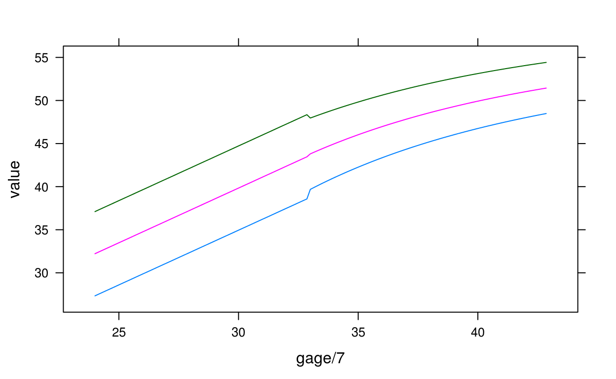
specific value to centile/z-score
Convert birth measurements to INTERGROWTH z-scores/centiles
Usage
igb_lencm2zscore(gagebrth, lencm, sex = "Female")
igb_wtkg2zscore(gagebrth, wtkg, sex = "Female")
igb_hcircm2zscore(gagebrth, hcircm, sex = "Female")
igb_lencm2centile(gagebrth, lencm, sex = "Female")
igb_wtkg2centile(gagebrth, wtkg, sex = "Female")
igb_hcircm2centile(gagebrth, hcircm, sex = "Female")
Arguments
- gagebrth
- gestational age at birth in days
- lencm
- length(cm) measurement(s) to convert
- sex
- “Male” or “Female”
- wtkg
- weight (kg) measurement(s) to convert
- hcircm
- head circumference (cm) measurement(s) to convert
Note
For gestational ages between 24 and 33 weeks, the INTERGROWTH very early preterm standard is used.
References
International standards for newborn weight, length, and head circumference by gestational age and sex: the Newborn Cross-Sectional Study of the INTERGROWTH-21st Project Villar, José et al. The Lancet, Volume 384, Issue 9946, 857-868
INTERGROWTH-21st very preterm size at birth reference charts. Lancet 2016 doi.org/10.1016/S0140-6736(16) 00384-6. Villar, José et al.
Examples
# get Male birth length z-scores
# first we need just 1 record per subject with subject-level data
cppsubj <- get_subject_data(cpp)
cppsubj <- subset(cppsubj, sex == "Male")
igb_lencm2zscore(cpp$gagebrth, cpp$birthlen, sex = "Male")
## [1] 2.57008863 2.57008863 2.57008863 0.66769390 0.66769390
## [6] 0.66769390 0.66769390 2.77551410 0.24012569 1.20761609
## [11] 0.43007110 1.53920598 1.53920598 1.53920598 1.53920598
## [16] 1.53920598 1.53920598 1.53920598 1.53920598 1.53920598
## [21] 2.57008863 2.57008863 2.57008863 2.57008863 2.57008863
## [26] NA NA 1.37080474 1.37080474 1.37080474
## [31] 2.08629993 2.08629993 2.08167545 2.08167545 2.08167545
## [36] -0.92887191 -0.92887191 -0.92887191 -0.92887191 -0.17659363
## [41] -0.17659363 -0.17659363 -0.17659363 -0.17659363 0.43007110
## [46] 0.43007110 0.43007110 0.43007110 0.04777744 0.04777744
## [51] 0.04777744 0.04777744 -0.95427104 -0.95427104 -0.95427104
## [56] -0.95427104 -0.95427104 0.04777744 0.04777744 0.04777744
## [61] 0.04777744 0.10144540 0.10144540 0.10144540 1.01947447
## [66] 1.01947447 1.01947447 1.01947447 1.26177582 1.26177582
## [71] 1.26177582 1.26177582 1.26177582 1.01947447 1.01947447
## [76] 1.01947447 1.01947447 1.01947447 0.04777744 0.04777744
## [81] 0.04777744 0.04777744 0.04777744 2.08629993 2.08629993
## [86] 2.08629993 2.08629993 0.43007110 0.43007110 0.43007110
## [91] 0.43007110 0.04777744 2.08629993 2.08629993 2.08629993
## [96] 0.81893628 0.81893628 0.81893628 1.01947447 1.01947447
## [101] 1.01947447 1.01947447 0.24012569 0.24012569 0.24012569
## [106] 0.24012569 0.94776774 0.94776774 0.94776774 0.94776774
## [111] 1.26326658 1.26326658 1.26326658 1.26326658 1.26326658
## [116] 0.04777744 0.04777744 0.04777744 0.04777744 0.66769390
## [121] 0.66769390 0.66769390 -0.17659363 -0.17659363 -0.17659363
## [126] -0.17659363 0.43007110 0.43007110 0.43007110 0.43007110
## [131] 1.57506493 1.57506493 1.57506493 1.57506493 -0.57693404
## [136] -0.57693404 -0.57693404 -0.57693404 -1.18192366 -1.18192366
## [141] -1.18192366 -1.18192366 -1.18192366 0.32057449 0.32057449
## [146] 0.32057449 0.32057449 -0.32198638 -0.32198638 -0.32198638
## [151] -0.32198638 -0.32198638 NA NA NA
## [156] 1.01947447 1.01947447 1.01947447 -0.32198638 -0.32198638
## [161] -0.32198638 -0.32198638 0.32057449 0.32057449 0.32057449
## [166] 0.43007110 0.43007110 0.43007110 1.84381500 1.84381500
## [171] 1.84381500 0.24012569 0.24012569 0.24012569 0.24012569
## [176] 1.88394745 1.88394745 1.88394745 1.88394745 1.88394745
## [181] -0.95427104 -0.95427104 -0.95427104 -0.95427104 -0.95427104
## [186] -0.32198638 -0.32198638 -0.32198638 -0.32198638 -0.32198638
## [191] 1.57506493 1.57506493 1.57506493 1.57506493 -0.57693404
## [196] -0.57693404 -0.57693404 -0.57693404 0.04777744 0.04777744
## [201] -1.88881195 -1.88881195 -1.88881195 -1.88881195 0.43007110
## [206] 0.43007110 0.43007110 -0.57693404 -0.57693404 -0.57693404
## [211] -0.57693404 0.10144540 0.10144540 0.10144540 2.54912777
## [216] 2.54912777 2.54912777 2.54912777 1.53920598 1.53920598
## [221] 1.53920598 1.53920598 -0.01724797 -0.01724797 -0.01724797
## [226] -0.01724797 -0.17659363 -0.17659363 -0.17659363 -0.17659363
## [231] 0.04777744 0.04777744 0.04777744 0.04777744 0.04777744
## [236] 2.31733522 2.31733522 2.31733522 2.31733522 2.31733522
## [241] 2.31733522 0.32057449 0.32057449 0.32057449 0.32057449
## [246] 0.32057449 0.32057449 1.53920598 1.53920598 1.53920598
## [251] 2.54912777 2.54912777 2.54912777 2.54912777 -1.02459617
## [256] -1.02459617 -1.02459617 -2.82067962 0.63678619 0.63678619
## [261] 0.63678619 0.63678619 0.66769390 0.66769390 0.66769390
## [266] 0.66769390 1.37080474 1.37080474 1.37080474 1.37080474
## [271] 0.24012569 0.24012569 0.24012569 0.24012569 3.15541741
## [276] 3.15541741 3.15541741 3.15541741 0.32057449 0.32057449
## [281] 0.32057449 0.32057449 -0.57693404 -0.57693404 -0.57693404
## [286] -0.57693404 0.24012569 0.24012569 0.24012569 0.24012569
## [291] 2.31733522 2.31733522 2.31733522 2.31733522 2.08167545
## [296] 2.08167545 2.08167545 2.08167545 1.53920598 1.53920598
## [301] 1.53920598 1.53920598 0.66769390 0.66769390 0.66769390
## [306] 0.66769390 0.66769390 1.81440917 1.81440917 1.81440917
## [311] 1.81440917 1.57506493 1.57506493 1.57506493 1.57506493
## [316] 1.26177582 1.26177582 1.26177582 1.26177582 1.26177582
## [321] 1.26177582 1.26177582 1.81440917 1.81440917 1.81440917
## [326] 1.81440917 1.81440917 1.26326658 1.26326658 1.26326658
## [331] 1.26326658 NA NA NA NA
## [336] -0.32198638 -0.32198638 -0.32198638 -0.32198638 2.35247762
## [341] 2.35247762 2.35247762 2.35247762 2.35247762 2.35247762
## [346] 2.35247762 2.35247762 2.35247762 2.08629993 2.08629993
## [351] 2.08629993 2.08629993 2.76890374 2.76890374 2.76890374
## [356] 2.76890374 2.08629993 2.08629993 2.08629993 2.08629993
## [361] 2.31733522 2.31733522 2.31733522 2.31733522 0.32057449
## [366] 0.32057449 0.32057449 0.32057449 0.04777744 -0.57693404
## [371] -0.57693404 1.26177582 1.26177582 1.26177582 1.26177582
## [376] -1.18192366 -1.18192366 -1.18192366 -1.18192366 0.94776774
## [381] 0.94776774 0.94776774 0.94776774 -0.95427104 -0.95427104
## [386] -0.95427104 -0.95427104 0.66523053 0.66523053 0.66523053
## [391] 0.66523053 0.66523053 -0.57693404 -0.57693404 -0.57693404
## [396] -0.57693404 -0.57693404 -0.17659363 -0.17659363 -0.17659363
## [401] -0.17659363 -0.34918388 -0.34918388 -0.34918388 -0.34918388
## [406] 2.31733522 2.31733522 2.31733522 -0.32198638 -0.32198638
## [411] -0.32198638 -0.32198638 0.04777744 0.04777744 0.04777744
## [416] 0.04777744 1.81440917 1.81440917 1.81440917 1.81440917
## [421] 0.94776774 0.94776774 0.94776774 0.94776774 0.43007110
## [426] 0.43007110 0.43007110 0.43007110 1.53920598 1.53920598
## [431] 1.53920598 1.53920598 1.53920598 NA NA
## [436] NA NA -0.57693404 -0.57693404 -0.57693404
## [441] -0.57693404 -0.77955940 -0.77955940 -0.77955940 -0.77955940
## [446] -0.77955940 0.24012569 0.24012569 0.24012569 0.24012569
## [451] 0.94776774 0.94776774 0.94776774 0.94776774 2.57008863
## [456] 2.57008863 2.57008863 2.57008863 2.57008863 1.01947447
## [461] 1.01947447 1.01947447 1.84381500 1.84381500 1.84381500
## [466] 1.57506493 1.57506493 1.57506493 1.57506493 -5.80376219
## [471] -5.80376219 -5.80376219 -5.80376219 2.76890374 2.76890374
## [476] 2.76890374 2.76890374 2.76890374 -0.77955940 -0.77955940
## [481] -0.77955940 -0.77955940 0.94776774 0.94776774 0.94776774
## [486] 0.94776774 1.53920598 1.53920598 1.53920598 1.53920598
## [491] 1.53920598 1.53920598 1.53920598 1.53920598 1.53920598
## [496] 1.53920598 -0.57693404 -0.57693404 -0.57693404 -0.57693404
## [501] 0.04777744 0.04777744 0.04777744 0.66769390 0.66769390
## [506] 0.66769390 0.66769390 0.66769390 1.37080474 1.37080474
## [511] 1.37080474 1.37080474 0.32057449 0.32057449 0.32057449
## [516] 0.32057449 0.66769390 0.66769390 0.66769390 0.66769390
## [521] 0.66769390 -1.18192366 -1.18192366 -1.18192366 -1.18192366
## [526] -5.39174617 -5.39174617 -5.39174617 -5.39174617 -5.39174617
## [531] -0.32198638 -0.32198638 -0.32198638 -2.10044386 -2.10044386
## [536] -2.10044386 1.81440917 1.81440917 1.81440917 1.81440917
## [541] 0.10144540 0.10144540 0.10144540 0.10144540 0.10144540
## [546] 2.31733522 2.31733522 2.31733522 2.31733522 0.04777744
## [551] 0.04777744 0.04777744 0.04777744 0.04777744 NA
## [556] NA NA NA 0.66769390 0.66769390
## [561] 0.66769390 0.32057449 0.32057449 0.32057449 1.26177582
## [566] 1.26177582 1.26177582 1.26177582 -0.32198638 -0.32198638
## [571] -0.32198638 -0.32198638 0.04777744 0.04777744 0.04777744
## [576] 0.04777744 NA -1.55221271 -1.55221271 -0.57693404
## [581] -0.57693404 -0.57693404 -0.57693404 0.94776774 -4.28567708
## [586] -4.28567708 -4.28567708 -4.28567708 -3.21277379 -3.21277379
## [591] -3.21277379 -3.21277379 -3.21277379 -1.74780621 -1.74780621
## [596] -1.74780621 -1.74780621 -0.67380818 -0.67380818 -0.67380818
## [601] -0.67380818 2.31733522 2.31733522 2.31733522 0.04777744
## [606] 0.04777744 0.04777744 0.04777744 -1.48019642 -1.48019642
## [611] -1.48019642 -1.48019642 1.26177582 1.26177582 1.26177582
## [616] 1.26177582 -0.95427104 -0.95427104 -0.95427104 0.32057449
## [621] 0.32057449 0.32057449 1.81440917 1.81440917 1.81440917
## [626] -1.74780621 -1.74780621 -1.74780621 NA 0.43007110
## [631] 0.43007110 0.43007110 0.43007110 -0.77955940 -0.77955940
## [636] -0.77955940 -0.77955940 -0.77955940 1.20761609 1.20761609
## [641] 1.20761609 1.20761609 1.20761609 -0.34918388 -0.34918388
## [646] -0.34918388 -0.34918388 0.81893628 0.81893628 0.81893628
## [651] 0.81893628 0.81893628 1.20761609 1.20761609 1.20761609
## [656] 1.20761609 1.20761609 1.26177582 1.26177582 1.26177582
## [661] -0.77955940 -0.77955940 -0.77955940 -0.77955940 1.01947447
## [666] 1.01947447 1.01947447 1.01947447 2.08167545 2.08167545
## [671] 2.08167545 2.08167545 1.84381500 1.84381500 1.84381500
## [676] 1.84381500 0.94776774 0.94776774 0.94776774 0.94776774
## [681] 2.76890374 2.76890374 0.04777744 1.81440917 1.81440917
## [686] 1.81440917 1.81440917 1.81440917 1.53920598 1.53920598
## [691] 1.53920598 1.53920598 -0.67380818 -0.67380818 -0.67380818
## [696] -0.67380818 0.04777744 0.04777744 0.04777744 0.94776774
## [701] 0.94776774 0.94776774 2.35247762 2.35247762 2.35247762
## [706] 2.35247762 -0.17659363 -0.17659363 -0.17659363 -0.17659363
## [711] 0.66769390 0.66769390 0.66769390 0.66769390 0.66769390
## [716] 2.08167545 2.08167545 2.08167545 2.08167545 0.32057449
## [721] 0.32057449 0.32057449 0.32057449 0.32057449 0.43007110
## [726] 0.43007110 0.43007110 0.43007110 NA NA
## [731] NA NA NA 2.76890374 2.76890374
## [736] 0.43007110 0.43007110 0.43007110 0.43007110 0.32057449
## [741] 0.32057449 0.32057449 0.32057449 -0.95427104 -0.95427104
## [746] -0.95427104 -0.95427104 -1.74780621 -1.74780621 -1.74780621
## [751] -1.74780621 0.66769390 0.66769390 0.66769390 0.66769390
## [756] 0.66769390 -1.35698291 -1.35698291 -1.35698291 -1.35698291
## [761] -1.35698291 NA NA NA NA
## [766] 2.54912777 2.54912777 2.54912777 2.54912777 2.54912777
## [771] NA -1.30459500 -1.30459500 -1.30459500 -1.30459500
## [776] 2.76890374 2.76890374 2.76890374 2.76890374 NA
## [781] NA NA NA NA 0.32057449
## [786] 0.32057449 0.32057449 0.32057449 0.32057449 1.53920598
## [791] 1.53920598 1.53920598 1.53920598 1.01947447 1.01947447
## [796] 1.01947447 1.01947447 1.01947447 2.96436156 2.96436156
## [801] 2.96436156 2.96436156 2.96436156 2.18498566 2.18498566
## [806] 2.18498566 0.66769390 0.66769390 0.66769390 0.66769390
## [811] 3.39217340 3.39217340 3.39217340 3.39217340 NA
## [816] NA NA NA 3.49617450 3.49617450
## [821] 3.49617450 3.49617450 3.49617450 1.26177582 1.26177582
## [826] 1.26177582 1.26177582 3.53071911 3.53071911 3.53071911
## [831] 3.53071911 3.53071911 1.71653479 1.71653479 1.71653479
## [836] 1.71653479 1.71653479 0.81893628 0.81893628 0.81893628
## [841] 0.81893628 0.81893628 3.33560617 3.33560617 3.33560617
## [846] 3.33560617 3.33560617 2.18498566 2.18498566 2.18498566
## [851] 2.18498566 -0.95427104 -0.95427104 -0.95427104 -0.95427104
## [856] 0.04777744 0.04777744 0.04777744 0.04777744 0.04777744
## [861] -2.10044386 -2.10044386 -2.10044386 0.66769390 0.66769390
## [866] 0.66769390 0.66769390 2.61075974 2.61075974 2.61075974
## [871] 2.61075974 2.61075974 0.24012569 0.24012569 0.24012569
## [876] 0.24012569 0.24012569 -0.17659363 -0.17659363 -0.17659363
## [881] -0.17659363 0.43007110 0.43007110 0.43007110 0.66769390
## [886] 0.66769390 0.66769390 0.66769390 0.04777744 0.04777744
## [891] 0.04777744 1.81440917 1.81440917 1.81440917 -1.18192366
## [896] -1.18192366 -1.18192366 -1.18192366 -0.17659363 -0.17659363
## [901] -0.17659363 -0.17659363 -0.17659363 2.35247762 2.35247762
## [906] 2.35247762 2.35247762 NA NA NA
## [911] NA NA -2.59359762 -2.59359762 -2.59359762
## [916] -2.59359762 -1.30459500 -1.30459500 -1.30459500 1.81440917
## [921] 1.81440917 1.81440917 1.81440917 1.81440917 0.66769390
## [926] 0.66769390 0.66769390 0.66769390 NA NA
## [931] NA NA 2.31733522 2.31733522 2.31733522
## [936] 2.31733522 1.57506493 1.57506493 1.57506493 1.57506493
## [941] 1.26177582 1.26177582 1.26177582 1.26177582 1.26177582
## [946] 2.08629993 2.08629993 2.08629993 0.43007110 0.43007110
## [951] 0.43007110 0.43007110 0.43007110 0.43007110 0.43007110
## [956] 0.43007110 -2.26398780 -2.26398780 -2.26398780 0.43007110
## [961] 0.43007110 0.43007110 0.43007110 0.66769390 0.66769390
## [966] 0.66769390 0.66769390 0.66769390 1.57506493 1.57506493
## [971] 1.57506493 1.57506493 1.57506493 1.26177582 1.26177582
## [976] 1.26177582 1.26177582 1.26177582 0.32057449 0.32057449
## [981] 0.32057449 0.66769390 0.66769390 0.66769390 0.66769390
## [986] 0.66769390 NA NA 1.26177582 1.26177582
## [991] 1.26177582 1.26177582 1.26177582 1.53920598 1.53920598
## [996] 1.53920598 1.53920598 0.04777744 0.04777744 0.04777744
## [1001] 0.04777744 0.04777744 0.04777744 0.04777744 0.04777744
## [1006] 0.04777744 0.63678619 0.63678619 0.63678619 0.63678619
## [1011] -0.77955940 -0.77955940 -0.77955940 -0.77955940 -0.77955940
## [1016] 0.43007110 0.43007110 0.43007110 0.43007110 1.26177582
## [1021] -0.17659363 -0.17659363 -0.17659363 -0.17659363 1.01947447
## [1026] 1.01947447 1.01947447 0.04777744 0.04777744 0.04777744
## [1031] 0.04777744 0.04777744 0.66769390 0.66769390 0.66769390
## [1036] 0.66769390 0.32057449 0.32057449 0.32057449 0.32057449
## [1041] 0.32057449 -0.32198638 -0.32198638 -0.32198638 -0.32198638
## [1046] -0.32198638 -1.18192366 -1.18192366 -1.18192366 -1.18192366
## [1051] 1.37080474 1.37080474 1.37080474 0.81893628 0.81893628
## [1056] 0.81893628 0.81893628 -0.17659363 2.76890374 -0.32198638
## [1061] -0.32198638 -0.32198638 -0.32198638 -2.26398780 -2.26398780
## [1066] -2.26398780 1.37080474 1.37080474 1.37080474 1.37080474
## [1071] -1.55209653 -1.55209653 -1.55209653 -1.55209653 -1.55209653
## [1076] 1.01947447 1.01947447 1.01947447 1.01947447 0.32057449
## [1081] 0.32057449 0.32057449 -0.34918388 1.01947447 1.01947447
## [1086] 1.01947447 1.01947447 1.81440917 1.81440917 0.94776774
## [1091] 1.20761609 0.43007110 0.43007110 0.43007110 0.43007110
## [1096] 0.94776774 0.94776774 0.94776774 0.66769390 0.66769390
## [1101] 0.66769390 0.66769390 0.66769390 2.08629993 2.08629993
## [1106] 2.08629993 -0.57693404 -0.57693404 -0.57693404 -0.57693404
## [1111] -0.92887191 -0.92887191 -0.92887191 1.37080474 1.37080474
## [1116] 1.37080474 1.37080474 2.96436156 2.96436156 2.96436156
## [1121] 2.96436156 2.96436156 2.57008863 2.57008863 2.57008863
## [1126] 2.57008863 1.81440917 1.81440917 1.81440917 1.81440917
## [1131] 1.81440917 0.04777744 0.04777744 0.04777744 0.04777744
## [1136] -2.72758934 -2.72758934 -2.72758934 -2.72758934 2.08167545
## [1141] 2.08167545 0.94776774 0.94776774 0.94776774 0.94776774
## [1146] 1.81440917 1.81440917 1.81440917 1.57506493 1.57506493
## [1151] -0.95427104 -0.95427104 -0.95427104 -0.95427104 -1.35698291
## [1156] -1.35698291 -1.35698291 -1.35698291 -1.55209653 -1.55209653
## [1161] -1.55209653 -1.55209653 -1.55209653 -1.55209653 -1.55209653
## [1166] -1.55209653 -1.55209653 0.04777744 0.04777744 0.04777744
## [1171] 0.04777744 0.04777744 0.81893628 0.81893628 0.81893628
## [1176] 0.81893628 0.81893628 0.66769390 0.66769390 0.66769390
## [1181] 0.66769390 1.81440917 1.81440917 1.81440917 1.81440917
## [1186] 1.81440917 1.88394745 1.88394745 1.88394745 1.88394745
## [1191] 1.71653479 1.71653479 1.71653479 1.71653479 0.66769390
## [1196] 0.66769390 0.66769390 -0.32198638 1.57506493 1.57506493
## [1201] 1.57506493 1.57506493 2.76890374 0.66769390 0.66769390
## [1206] -0.34918388 -0.34918388 -0.34918388 -0.34918388 -0.34918388
## [1211] -0.34918388 -0.34918388 -0.34918388 NA NA
## [1216] NA NA -0.77955940 -0.77955940 -0.77955940
## [1221] -0.77955940 0.32057449 0.24012569 0.24012569 0.24012569
## [1226] 0.24012569 1.37080474 1.37080474 1.37080474 1.26177582
## [1231] 1.26177582 1.26177582 2.76890374 2.76890374 2.76890374
## [1236] 2.76890374 0.04777744 0.04777744 0.04777744 0.04777744
## [1241] 1.57506493 1.57506493 1.57506493 1.57506493 1.57506493
## [1246] -0.77955940 -0.77955940 -0.77955940 -0.77955940 0.43007110
## [1251] 0.43007110 0.43007110 0.43007110 0.43007110 2.57008863
## [1256] 2.57008863 2.57008863 2.57008863 2.57008863 -0.77955940
## [1261] -0.77955940 -0.77955940 -0.77955940 -0.77955940 0.43007110
## [1266] 0.43007110 0.43007110 0.43007110 0.32057449 0.32057449
## [1271] 1.26177582 1.26177582 -0.17659363 -0.17659363 -0.17659363
## [1276] -1.35698291 -1.35698291 -1.35698291 -1.35698291 0.94776774
## [1281] 0.94776774 0.94776774 0.94776774 NA NA
## [1286] NA NA NA NA NA
## [1291] NA NA 1.01947447 1.01947447 1.01947447
## [1296] 1.01947447 -0.17659363 -0.17659363 -0.17659363 -0.92887191
## [1301] -0.92887191 -0.92887191 -0.92887191 -0.92887191 1.01947447
## [1306] 1.01947447 1.01947447 1.01947447 1.37080474 1.37080474
## [1311] 1.37080474 1.37080474 1.37080474 -0.95427104 -0.95427104
## [1316] -0.95427104 -0.95427104 0.66769390 0.66769390 0.66769390
## [1321] 0.66769390 0.66769390 -0.32198638 -0.32198638 -0.32198638
## [1326] -0.32198638 2.08629993 2.08629993 2.08629993 1.26177582
## [1331] 2.08167545 2.08167545 2.08167545 2.08167545 -1.48019642
## [1336] -1.48019642 -1.48019642 -1.30459500 -1.30459500 -1.30459500
## [1341] -1.30459500 2.57008863 2.57008863 2.57008863 2.57008863
## [1346] 2.57008863 1.81440917 1.81440917 1.81440917 1.81440917
## [1351] -0.01724797 -0.01724797 -0.01724797 0.66769390 0.66769390
## [1356] 0.66769390 0.66769390 1.26177582 1.26177582 1.26177582
## [1361] 1.26177582 1.01947447 1.01947447 1.01947447 1.01947447
## [1366] 1.01947447 2.08629993 2.08629993 2.08629993 2.08629993
## [1371] -0.17659363 -0.17659363 -0.17659363 -0.17659363 -0.17659363
## [1376] -0.17659363 -0.17659363 -0.17659363 -0.17659363 -0.67380818
## [1381] -0.67380818 -0.67380818 -0.67380818 -1.18192366 -1.18192366
## [1386] -1.18192366 -1.18192366 0.66769390 0.66769390 0.66769390
## [1391] 0.66769390 3.85113993 3.85113993 3.85113993 3.85113993
## [1396] 3.85113993 -2.38186551 -2.38186551 -2.38186551 -2.38186551
## [1401] -1.48019642 -1.48019642 -1.48019642 -1.48019642 -1.48019642
## [1406] 0.66769390 1.20761609 1.20761609 1.20761609 1.20761609
## [1411] -0.17659363 -0.17659363 -0.17659363 -0.17659363 -0.77955940
## [1416] -0.77955940 -0.77955940 -0.77955940 2.57008863 2.57008863
## [1421] 2.57008863 2.57008863 2.35247762 2.35247762 2.35247762
## [1426] 2.35247762 2.35247762 -2.59359762 -2.59359762 -2.59359762
## [1431] -0.57693404 -0.57693404 -0.57693404 -0.57693404 -0.57693404
## [1436] 2.57008863 2.57008863 2.57008863 2.57008863 -0.17659363
## [1441] -0.17659363 -0.17659363 -0.17659363 -0.17659363 2.08167545
## [1446] 2.08167545 2.08167545 2.36901940 2.36901940 2.36901940
## [1451] 2.36901940 1.88394745 1.88394745 1.88394745 1.88394745
## [1456] 2.96436156 2.96436156 2.96436156 2.96436156 2.96436156
## [1461] 2.31733522 2.31733522 2.31733522 1.81440917 1.81440917
## [1466] 1.81440917 1.84381500 1.84381500 1.84381500 1.84381500
## [1471] 1.26177582 1.26177582 1.26177582 1.26177582 1.57506493
## [1476] 1.57506493 1.57506493 1.57506493 -0.67380818 -0.67380818
## [1481] -0.67380818 -0.67380818 0.66523053 0.66523053 0.66523053
## [1486] 0.66523053 0.66523053 -0.32198638 -0.32198638 -0.32198638
## [1491] -2.10044386 -2.10044386 -2.10044386 -2.10044386 -0.77955940
## [1496] -0.77955940 -0.77955940 -0.77955940 -0.77955940 NA
## [1501] NA NA NA 1.26177582 1.26177582
## [1506] 1.26177582 2.08629993 2.08629993 2.08629993 2.08629993
## [1511] NA NA NA NA -1.18192366
## [1516] -1.18192366 -1.18192366 -1.18192366 3.00545515 3.00545515
## [1521] 3.00545515 3.00545515 3.00545515 1.88394745 1.88394745
## [1526] 1.88394745 1.88394745 1.37080474 1.37080474 1.37080474
## [1531] 1.37080474 1.37080474 1.01947447 1.01947447 1.01947447
## [1536] -0.34918388 -0.34918388 -0.34918388 -0.34918388 -0.34918388
## [1541] 1.53920598 1.53920598 1.53920598 1.53920598 2.54912777
## [1546] 2.54912777 2.54912777 2.54912777 0.32057449 0.32057449
## [1551] 0.32057449 0.32057449 NA NA NA
## [1556] NA 0.43007110 0.43007110 0.43007110 0.43007110
## [1561] -0.17659363 -0.17659363 -0.17659363 -0.17659363 -0.17659363
## [1566] -0.32198638 -0.32198638 -0.32198638 -0.32198638 -0.32198638
## [1571] 1.81440917 1.81440917 1.81440917 1.81440917 1.81440917
## [1576] -0.57693404 -0.57693404 -0.57693404 -0.57693404 0.66769390
## [1581] 0.66769390 0.66769390 0.66769390 4.04258904 4.04258904
## [1586] 4.04258904 4.04258904 4.04258904 -1.55209653 -1.55209653
## [1591] -1.55209653 -1.55209653 2.77551410 2.77551410 2.77551410
## [1596] 0.66769390 0.66769390 0.66769390 0.66769390 -0.67380818
## [1601] -0.67380818 -0.67380818 -0.67380818 -0.67380818 1.01947447
## [1606] 1.01947447 1.01947447 1.01947447 1.01947447 2.31733522
## [1611] 2.31733522 2.31733522 2.31733522 2.76890374 2.76890374
## [1616] 2.76890374 2.76890374 2.76890374 1.37080474 1.37080474
## [1621] 1.37080474 0.63678619 0.63678619 0.63678619 0.63678619
## [1626] 0.63678619 1.88394745 1.88394745 1.88394745 -1.18192366
## [1631] -1.18192366 -1.18192366 1.01947447 1.01947447 0.43007110
## [1636] 0.43007110 0.43007110 0.66769390 0.66769390 1.53920598
## [1641] 1.53920598 1.53920598 1.53920598 1.57506493 1.57506493
## [1646] 1.57506493 1.57506493 1.57506493 0.66769390 0.66769390
## [1651] 0.66769390 1.37080474 1.37080474 1.37080474 1.37080474
## [1656] -0.92887191 -0.92887191 -0.92887191 -0.92887191 -0.92887191
## [1661] -0.57693404 -0.57693404 -0.57693404 -0.57693404 2.08167545
## [1666] 2.08167545 2.08167545 2.08167545 0.43007110 0.43007110
## [1671] 0.43007110 0.43007110 -1.18192366 -1.18192366 -1.18192366
## [1676] -1.18192366 1.84381500 1.84381500 1.84381500 1.84381500
## [1681] 1.37080474 1.57506493 1.57506493 1.57506493 0.43007110
## [1686] 0.43007110 1.26177582 1.26177582 1.26177582 1.26177582
## [1691] -0.17659363 -0.17659363 -0.17659363 -0.17659363 -0.92887191
## [1696] -0.92887191 -0.92887191 -0.92887191 1.88394745 1.88394745
## [1701] 1.88394745 0.04777744 0.04777744 0.04777744 0.04777744
## [1706] NA NA NA -0.17659363 -0.17659363
## [1711] -0.17659363 -0.01724797 -0.01724797 0.43007110 0.43007110
## [1716] 0.43007110 0.43007110 1.20761609 1.20761609 1.20761609
## [1721] 1.20761609 1.20761609 -1.30459500 -1.30459500 -1.30459500
## [1726] -1.30459500 -1.30459500 1.53920598 1.53920598 1.53920598
## [1731] -0.17659363 -0.17659363 -0.17659363 -0.17659363 -0.17659363
## [1736] 0.66769390 0.66769390 0.66769390 0.66769390 0.66769390
## [1741] -0.01724797 -0.01724797 -0.01724797 -0.01724797 -0.32198638
## [1746] -0.32198638 -0.32198638 -0.32198638 0.32057449 0.32057449
## [1751] 0.32057449 0.32057449 0.32057449 NA -2.87419725
## [1756] -2.87419725 -2.87419725 -0.77955940 -0.77955940 -0.77955940
## [1761] -0.77955940 0.24012569 0.24012569 0.24012569 0.24012569
## [1766] -0.32198638 -0.32198638 -0.32198638 -0.32198638 -0.32198638
## [1771] 0.32057449 0.32057449 0.32057449 0.32057449 -0.77955940
## [1776] -0.77955940 -0.77955940 -0.77955940 -0.77955940 3.39217340
## [1781] 3.39217340 3.39217340 3.39217340 3.39217340 3.33560617
## [1786] 3.33560617 3.33560617 3.33560617 3.33560617 3.17177418
## [1791] 3.17177418 3.17177418 3.17177418 -1.35698291 -1.35698291
## [1796] -1.35698291 -1.35698291 0.04777744 0.04777744 0.04777744
## [1801] 0.04777744 0.04777744 1.37080474 1.37080474 1.37080474
## [1806] 1.37080474 0.43007110 0.43007110 0.43007110 0.43007110
## [1811] 2.54912777 2.54912777 2.54912777 2.54912777 2.54912777
## [1816] 2.54912777 2.54912777 2.54912777 2.54912777 2.54912777
## [1821] 0.94776774 0.94776774 0.94776774 0.94776774 2.36901940
## [1826] 2.36901940 2.36901940 2.36901940 -0.95427104 -0.95427104
## [1831] -0.95427104 -0.95427104 0.63678619 0.63678619 0.63678619
## [1836] 0.63678619 0.63678619 2.57008863 2.57008863 2.57008863
## [1841] 2.57008863 2.57008863 0.63678619 0.63678619 0.63678619
## [1846] 0.63678619 0.63678619 1.57506493 1.57506493 1.57506493
## [1851] 1.57506493 0.94776774 0.94776774 0.94776774 0.94776774
## [1856] 0.04777744 0.04777744 0.04777744 -0.57693404 -0.57693404
## [1861] -0.57693404 -0.57693404 -0.17659363 -0.17659363 -0.17659363
## [1866] -0.17659363 -1.18192366 -1.18192366 -1.18192366 -1.18192366
## [1871] -1.35698291 -1.35698291 -1.35698291 -1.35698291 0.63678619
## [1876] 0.63678619 0.63678619 0.63678619 0.94776774 0.94776774
## [1881] 0.94776774 0.94776774 0.94776774 -2.10044386 -2.10044386
## [1886] -2.10044386 -2.10044386 0.04777744 0.04777744 1.26177582
## [1891] 1.26177582 1.26177582 1.26177582 1.01947447 1.01947447
## [1896] 1.01947447 1.53920598 1.53920598 1.53920598 1.53920598
## [1901] 1.81440917 1.81440917 1.81440917 1.81440917 1.81440917
## [1906] 0.94776774 0.94776774 0.94776774 0.94776774 -2.59359762
## [1911] -2.59359762 -2.59359762Intergrowth Fetal Standards
generic centile/z-score to value
Convert INTERGROWTH z-scores/centiles to fetal ultrasound measurements (generic)
Usage
igfet_zscore2value(gagedays, z = 0, var = c("hccm", "bpdcm", "ofdcm", "accm", "flcm"))
igfet_centile2value(gagedays, p = 50, var = c("hccm", "bpdcm", "ofdcm", "accm", "flcm"))
Arguments
- gagedays
- gestational age in days
- z
- z-score(s) to convert
- var
- the name of the measurement to convert (“hccm”, “bpdcm”, “ofdcm”, “accm”, “flcm”)
- p
- centile(s) to convert (must be between 0 and 100)
References
International standards for fetal growth based on serial ultrasound measurements: the Fetal Growth Longitudinal Study of the INTERGROWTH-21st Project Papageorghiou, Aris T et al. The Lancet, Volume 384, Issue 9946, 869-879
Examples
# get value for median head circumference for child at 100 gestational days
igfet_centile2value(100, 50, var = "hccm")
## [1] 10.14404generic value to centile/z-score
Convert fetal ultrasound measurements to INTERGROWTH z-scores/centiles (generic)
Usage
igfet_value2zscore(gagedays, val, var = c("hccm", "bpdcm", "ofdcm", "accm", "flcm"))
igfet_value2centile(gagedays, val, var = c("hccm", "bpdcm", "ofdcm", "accm", "flcm"))
Arguments
- gagedays
- gestational age in days
- val
- the value(s) of the anthro measurement to convert
- var
- the name of the measurement to convert (“hccm”, “bpdcm”, “ofdcm”, “accm”, “flcm”)
References
International standards for fetal growth based on serial ultrasound measurements: the Fetal Growth Longitudinal Study of the INTERGROWTH-21st Project Papageorghiou, Aris T et al. The Lancet, Volume 384, Issue 9946, 869-879
Examples
# get centile for child at 100 gestational days with 11 cm head circumference
igfet_hccm2centile(100, 11)
## [1] 93.39812specific centile/z-score to value
Convert INTERGROWTH z-scores/centiles to fetal ultrasound measurements
Usage
igfet_zscore2hccm(gagedays, z = 0)
igfet_zscore2bpdcm(gagedays, z = 0)
igfet_zscore2ofdcm(gagedays, z = 0)
igfet_zscore2accm(gagedays, z = 0)
igfet_zscore2flcm(gagedays, z = 0)
igfet_centile2hccm(gagedays, p = 50)
igfet_centile2bpdcm(gagedays, p = 50)
igfet_centile2ofdcm(gagedays, p = 50)
igfet_centile2accm(gagedays, p = 50)
igfet_centile2flcm(gagedays, p = 50)
Arguments
- gagedays
- gestational age in days
- z
- z-score(s) to convert
- p
- centile(s) to convert (must be between 0 and 100)
References
International standards for fetal growth based on serial ultrasound measurements: the Fetal Growth Longitudinal Study of the INTERGROWTH-21st Project Papageorghiou, Aris T et al. The Lancet, Volume 384, Issue 9946, 869-879
Examples
# get value for median head circumference for child at 100 gestational days
igfet_centile2hccm(100, 50)
## [1] 10.14404specific value to centile/z-score
Convert fetal ultrasound measurements to INTERGROWTH z-scores/centiles
Usage
igfet_hccm2zscore(gagedays, hccm)
igfet_bpdcm2zscore(gagedays, bpdcm)
igfet_ofdcm2zscore(gagedays, ofdcm)
igfet_accm2zscore(gagedays, accm)
igfet_flcm2zscore(gagedays, flcm)
igfet_hccm2centile(gagedays, hccm)
igfet_bpdcm2centile(gagedays, bpdcm)
igfet_ofdcm2centile(gagedays, ofdcm)
igfet_accm2centile(gagedays, accm)
igfet_flcm2centile(gagedays, flcm)
Arguments
- gagedays
- gestational age in days
- hccm
- head circumference (cm) measurement(s) to convert
- bpdcm
- biparietel diameter (cm) measurement(s) to convert
- ofdcm
- occipito-frontal diameter (cm) measurement(s) to convert
- accm
- abdominal circumference (cm) measurement(s) to convert
- flcm
- femur length (cm) measurement(s) to convert
References
International standards for fetal growth based on serial ultrasound measurements: the Fetal Growth Longitudinal Study of the INTERGROWTH-21st Project Papageorghiou, Aris T et al. The Lancet, Volume 384, Issue 9946, 869-879
Examples
# get centile for child at 100 gestational days with 11 cm head circumference
igfet_hccm2centile(100, 11)
## [1] 93.39812Growth Standard Vis
Growth standard methods
Utility functions for adding growth standard bands to rbokeh/lattice/ggplot2 plots
Usage
panel.who(x, x_var = "agedays", y_var = "htcm", sex = "Female", p = c(1, 5, 25, 50), color = NULL, alpha = 0.15, center = FALSE, labels = TRUE, x_trans = identity, y_trans = identity)
panel.igb(gagebrth, var = "lencm", sex = "Female", p = c(1, 5, 25, 50), color = NULL, alpha = 0.15, center = FALSE, labels = TRUE, x_trans = identity, y_trans = identity)
panel.igfet(gagedays, var = "hccm", p = c(1, 5, 25, 50), color = "green", alpha = 0.15, center = FALSE, labels = TRUE, x_trans = identity, y_trans = identity)
geom_growthstandard(mapping = NULL, data = NULL, x_seq, x_var = "agedays", y_var, sex = "Female", p = c(1, 5, 25, 50), shade = NULL, alpha = 0.15, center = FALSE, x_trans = identity, y_trans = identity, standard = "who", inherit.aes = TRUE)
geom_who(...)
geom_igb(..., var = "lencm")
geom_igfet(..., var = "hccm", color = "green")
ly_who(fig, x, x_var = "agedays", y_var = "htcm", sex = "Female", p = c(1, 5, 25, 50), color = NULL, alpha = 0.15, center = FALSE, labels = TRUE, x_trans = identity, y_trans = identity, x_units = c("days", "months", "years"))
ly_igb(fig, gagebrth, var = "lencm", sex = "Female", p = c(1, 5, 25, 50), color = NULL, alpha = 0.15, center = FALSE, labels = TRUE, x_trans = identity, y_trans = identity)
ly_igfet(fig, gagedays, var = "hccm", p = c(1, 5, 25, 50), color = "green", alpha = 0.15, center = FALSE, labels = TRUE, x_trans = identity, y_trans = identity)
Arguments
- x, x_seq
-
value or vector of values that correspond to a measure defined by
x_var.x_seqis used with geom_* - x_var
- x variable name (typically “agedays”)
- y_var
- y variable name (typically “htcm” or “wtkg”)
- sex
- “Male” or “Female”
- p
- centiles at which to draw the growth standard band polygons (only need to specify on one side of the median)
- color, shade
-
optional color to use for bands (will use
sexto determine if not specified).shadeis used with geom_* - alpha
- transparency of the bands
- center
- should the bands be centered around the median?
- labels
- should the centiles be labeled? (not implemented)
- x_trans
- transformation function to be applied to x-axis
- y_trans
- transformation function to be applied to y-axis
- gagebrth
- gestational age at birth in days (for igb plots)
- var
- variable name for y axis for igb or igfet plots (“lencm”, “wtkg”, or “hcircm” for igb; “accm”, “bpdcm”, “flcm”, “hccm”, or “ofdcm” for igfet)
- gagedays
- gestational age in days (for igfet plots)
- data, mapping, inherit.aes
-
supplied direclty to
ggplot2::layer - standard
-
standard name to use. Either
“who”,“igb”, or“igfet” - …
-
items supplied direclty to
geom_growthstandard - fig
- rbokeh figure to add growth standard to
- x_units
- units of age x-axis (days, months, or years)
Examples
## Not run:
# #### rbokeh
#
# library(rbokeh)
# figure() %>%
#   ly_who(x = seq(0, 2558, by = 30), y_var = "wtkg",
#     x_trans = days2years, sex = "Male") %>%
#   ly_points(days2years(agedays), wtkg,
#     data = subset(cpp, subjid == 8), col = "black",
#     hover = c(agedays, wtkg, lencm, htcm, bmi, geniq, sysbp, diabp))
#
# cpp$wtkg50 <- who_centile2value(cpp$agedays, y_var = "wtkg")
# figure() %>%
#   ly_who(x = seq(0, 2558, by = 30), y_var = "wtkg", color = "blue",
#     x_trans = days2years, center = TRUE) %>%
#   ly_points(days2years(agedays), wtkg - wtkg50, color = "black",
#     data = subset(cpp, subjid == 8))
#
# # look at Male birth lengths superposed on INTERGROWTH birth standard
# # first we need just 1 record per subject with subject-level data
# cppsubj <- get_subject_data(cpp)
# figure(xlab = "Gestational Age at Birth (days)", ylab = "Birth Length (cm)") %>%
#   ly_igb(gagebrth = 250:310, var = "lencm", sex = "Male") %>%
#   ly_points(jitter(gagebrth), birthlen, data = subset(cppsubj, sex == "Male"),
#     color = "black")
#
# # plot growth standard bands at z=1, 2, 3 for fetal head circumference
# figure(xlab = "Gestational Age (days)",
#   ylab = "Head Circumference (cm)") %>%
#     ly_igfet(gagedays = 98:280, var = "hccm", p = pnorm(-3:0) * 100)
# ## End(Not run)

#### lattice

library(lattice)
xyplot(wtkg ~ agedays, data = subset(cpp, subjid == 8),
  panel = function(x, y, ...) {
    panel.who(x = seq(0, 2558, by = 30),
      sex = "Male", y_var = "wtkg", p = 100 * pnorm(-3:0))
    panel.xyplot(x, y, ...)
  },
  col = "black"
)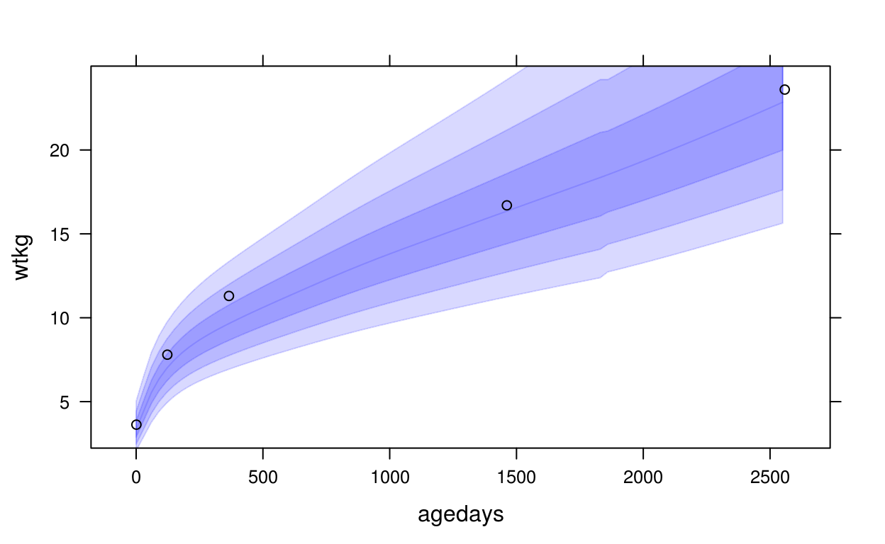
# look at Male birth lengths superposed on INTERGROWTH birth standard
# first we need just 1 record per subject with subject-level data
cppsubj <- get_subject_data(cpp)
xyplot(birthlen ~ jitter(gagebrth), data = subset(cppsubj, sex == "Male"),
  panel = function(x, y, ...) {
    panel.igb(gagebrth = 250:310, var = "lencm", sex = "Male")
    panel.points(x, y, ...)
  },
  col = "black", alpha = 0.75,
  xlab = "Gestational Age at Birth (days)", ylab = "Birth Length (cm)"
)
#### ggplot2

library(ggplot2)
p <- ggplot(data = subset(cpp, subjid == 8), aes(x = agedays, y = htcm)) +
  geom_who(x_seq = seq(0, 2600, by = 10), y_var = "htcm") +
  geom_point()
z-score scale methods
Utility functions for adding growth standard bands to rbokeh/lattice/ggplot2 plots
Usage
ly_zband(fig, x, z = -3:0, color = "green", alpha = 0.15, x_units = c("days", "months", "years"))
panel.zband(x, z = -3:0, color = "green", alpha = 0.25)
geom_zband(obj, x, z = -3:0, color = "green", alpha = 0.25)
Arguments
- fig
- rbokeh figure to add z bands to
- x
- range on x axis that should be covered by bands
- z
- z-scores at which to draw bands (only need to specify on one side of zero)
- color
- color to use for bands
- alpha
- transparency of the bands
- x_units
- units of age x-axis (days, months, or years)
- obj
- ggplot2 object to add z bands to
Examples
## Not run:
# library(rbokeh)
# figure() %>%
#   ly_zband(cpp$agedays) %>%
#   ly_points(jitter(agedays), haz, data = cpp, color = "black")
#
# library(lattice)
# xyplot(haz ~ jitter(agedays), data = cpp,
#   panel = function(x, y, ...) {
#     panel.zband(x)
#     panel.xyplot(x, y, ...)
#   },
#   col = "black", alpha = 0.5
# )
#
# library(ggplot2)
# p <- ggplot(data = cpp, aes(x = jitter(agedays), y = haz))
# geom_zband(p, x = seq(0, 2600, by = 10)) +
#   geom_point()
# ## End(Not run)
Modeling
get_fit
Obtain a trajectory “fit” object for a dataset
Usage
get_fit(dat, x_var = "agedays", y_var = "htcm", method = "fda", holdout = FALSE, x_trans = NULL, x_inv = NULL, y_trans = NULL, y_inv = NULL, ...)Arguments
- dat
- data frame containing variables to model
- x_var
- name of x variable to model (default is “agedays”)
- y_var
- name of y variable to model (usually an anthropometric measure or z-score scaled anthropometric measure)
- method
-
name of fitting method to use (see
get_avail_methods) - holdout
-
should an observation be held out for fitting (will use column
holdindatto which observations to hold out) - x_trans, y_trans
- transformation functions to be applied to x and y prior to modeling
- x_inv, y_inv
- inverse transformation functions for x and y to get back to the original scale after modeling
- …
- parameters passed on to the fitting method
fit_trajectory
Apply a model fit to an individual’s trajectory
Usage
fit_trajectory(dat, fit, xg = NULL, checkpoints = 365 * c(1:2), z_bins = -2)Arguments
- dat
- data frame containing variables for one subject to apply a fit to
- fit
-
an object returned from
get_fit - xg
-
grid of x points at which the fit should be evaluated for plotting (if
NULLit will be set to an equally-spaced grid of 150 points acrossx) - checkpoints
- x values at which to compute “checkpoints” of the subjectss growth trajectory to compare to other subjects
- z_bins
- a vector indicating binning of z-scores for the subjects trajectory at each checkpoint with respect to the the WHO growth standard
Examples
mod <- get_fit(cpp, y_var = "wtkg")
fit <- fit_trajectory(subset(cpp, subjid == 2), mod)
plot(fit$xy$x, fit$xy$y)
lines(fit$fitgrid$x, fit$fitgrid$y)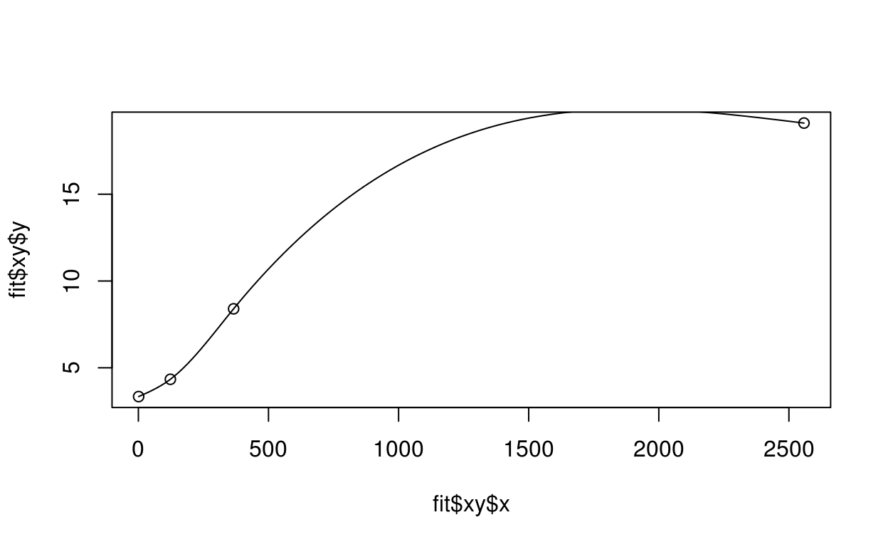
# there is also a plot method:
plot(fit, x_range = c(0, 2560))
# we can fit the z-scores instead
mod2 <- get_fit(cpp, y_var = "waz")
fit2 <- fit_trajectory(subset(cpp, subjid == 2), mod2)## some z-scores were too large - setting to 8plot(fit2$xy$x, fit2$xy$z)
lines(fit2$fitgrid$x, fit2$fitgrid$z)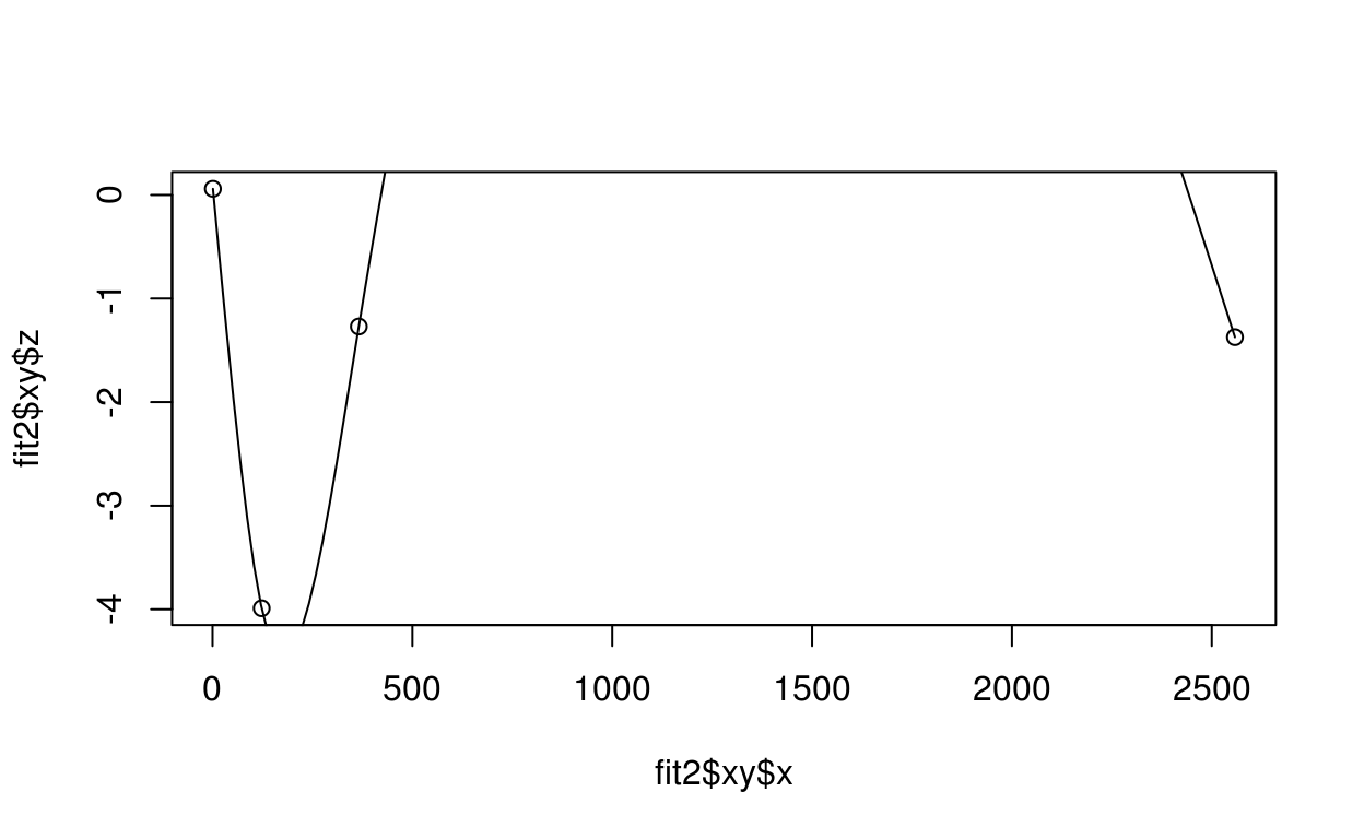
# using the plot method
plot(fit2, x_range = c(0, 2560), center = TRUE)
fit_all_trajectories
Apply trajectory fitting to each subject in a dataset
Usage
fit_all_trajectories(dat, fit, xg = NULL, checkpoints = 365 * c(1:2), z_bins = -2)Arguments
- dat
-
a data frame containing data for several subjects or a ddf already divided by subject, as obtained from
by_subject - fit
-
an object returned from
get_fit - xg
-
grid of x points at which the fit should be evaluated for plotting (if
NULLit will be set to an equally-spaced grid of 150 points acrossx) - checkpoints
- x values at which to compute “checkpoints” of the subjectss growth trajectory to compare to other subjects
- z_bins
- a vector indicating binning of z-scores for the subjects trajectory at each checkpoint with respect to the the WHO growth standard
Examples
## Not run:
# cppfit <- get_fit(cpp, y_var = "wtkg", method = "rlm")
# cpptr  <- fit_all_trajectories(cpp, cppfit)
# cpptr[[1]]
# plot(cpptr[[1]]$value)
# ## End(Not run)
get_fit_holdout_mse
Get MSE for holdout
Usage
get_fit_holdout_mse(d, z = TRUE)Arguments
- d
-
an object returned from
fit_all_trajectories - z
- compute MSE on z-score scale or original scale?
get_fit_holdout_errors
Get holdout errors
Usage
get_fit_holdout_errors(d, z = TRUE)Arguments
- d
-
an object returned from
fit_all_trajectories - z
- compute MSE on z-score scale or original scale?
plot.fittedTrajectory
Plot a fitted trajectory
Usage
"plot"(x, center = FALSE, x_range = NULL, width = 500, height = 520, hover = NULL, checkpoints = TRUE, p = 100 * pnorm(-3:0), x_units = c("days", "months", "years"), ...)Arguments
- x
-
an object returned from
fit_trajectory - center
- should the trajectory be centered around the median WHO standard? This is equivalent to plotting the age difference score (like height-for-age difference - HAD)
- x_range
- a vector specifying the range (min, max) that the superposed growth standard should span on the x-axis
- width
- width of the plot
- height
- height of the plot
- hover
-
variable names in
x$datato show on hover for each point (only variables with non-NA data will be shown) - checkpoints
- should the checkpoints be plotted (if available)?
- p
- centiles at which to draw the WHO polygons
- x_units
- units of age x-axis (days, months, or years)
- …
-
additional parameters passed to
figure
Examples
mod <- get_fit(cpp, y_var = "wtkg", method = "rlm")
fit <- fit_trajectory(subset(cpp, subjid == 2), mod)
plot(fit)
plot(fit, x_units = "years")plot(fit, center = TRUE)plot(fit, hover = c("wtkg", "bmi", "waz", "haz"))plot_z
Plot a fitted trajectory on z-score scale
Usage
plot_z(x, x_range = NULL, nadir = FALSE, recovery = NULL, width = 500, height = 520, hover = NULL, checkpoints = TRUE, z = -3:0, x_units = c("days", "months", "years"), ...)Arguments
- x
-
an object returned from
fit_trajectory - x_range
- a vector specifying the range (min, max) that the superposed z-score bands should span on the x-axis
- nadir
- should a guide be added to the plot showing the location of the nadir?
- recovery
- age in days at which to plot recovery from nadir (only valid if nadir is TRUE) - if NULL (default), will not be plotted
- width
- width of the plot
- height
- height of the plot
- hover
-
variable names in
x$datato show on hover for each point (only variables with non-NA data will be shown) - checkpoints
- should the checkpoints be plotted (if available)?
- z
- z-scores at which to draw the z-score bands
- x_units
- units of age x-axis (days, months, or years)
- …
-
additional parameters passed to
figure
Examples
mod <- get_fit(cpp, y_var = "wtkg", method = "rlm")
fit <- fit_trajectory(subset(cpp, subjid == 2), mod)
plot_z(fit)
plot_velocity
Plot a fitted trajectory’s velocity
Usage
plot_velocity(x, width = 500, height = 520, x_units = c("days", "months", "years"), ...)Arguments
- x
-
an object returned from
fit_trajectory - width
- width of the plot
- height
- height of the plot
- x_units
- units of age x-axis (days, months, or years)
- …
-
additional parameters passed to
figure
Examples
mod <- get_fit(cpp, y_var = "wtkg", method = "rlm")
fit <- fit_trajectory(subset(cpp, subjid == 2), mod)
plot_velocity(fit)
plot_zvelocity
Plot a fitted trajectory’s z-score velocity
Usage
plot_zvelocity(x, width = 500, height = 520, x_units = c("days", "months", "years"), ...)Arguments
- x
-
an object returned from
fit_trajectory - width
- width of the plot
- height
- height of the plot
- x_units
- units of age x-axis (days, months, or years)
- …
-
additional parameters passed to
figure
Examples
mod <- get_fit(cpp, y_var = "wtkg", method = "rlm")
fit <- fit_trajectory(subset(cpp, subjid == 2), mod)
plot_zvelocity(fit)fit_method.brokenstick
Get the result of fitting brokenstick to a dataset
Usage
"fit_method"(dat, ...)Arguments
- dat
- data frame containing variables to model
- …
-
additional parameters passed to
brokenstick, most notablyknots
Details
This essentially gets an anthropometric dataset into shape for brokenstick (sets appropriate data structure and removes missing values) and runs the fitting routine.
Note
The settings for x_trans and y_trans must match that used in fit_trajectory and appropriate inverse transformations must be set there accordingly as well.
Examples
## Not run:
# bsfit <- get_fit(cpp, y_var = "haz", method = "brokenstick")
# fit <- fit_trajectory(subset(cpp, subjid == 2), fit = bsfit)
# plot(fit)
# ## End(Not run)
fit_method.face
Get the result of fitting face.sparse to a dataset
Usage
"fit_method"(dat, ...)Arguments
- dat
- data frame containing variables to model
- …
-
additional parameters passed to
face.sparse, most notablyknotswhich defaults to 10
Details
This essentially gets an anthropometric dataset into shape for face.sparse (sets appropriate data structure and removes missing values) and runs the fitting routine.
Note
The settings for x_trans and y_trans must match that used in fit_trajectory and appropriate inverse transformations must be set there accordingly as well.
Examples
## Not run:
# facefit <- get_fit(cpp, y_var = "haz", method = "face")
# fit <- fit_trajectory(subset(cpp, subjid == 2), fit = facefit)
# plot(fit)
# ## End(Not run)
fit_method.fda
Compute functional “fda” fit of growth trajectory
Usage
"fit_method"(dat, ...)Arguments
- dat
- data frame specifying x and y coordinates of data to fit
- …
-
additional parameters passed to
smooth.basisPar, notablylambdawhich defaults to 0.1
Note
The trajectory fitting functions are most easily accessed through calling fit_trajectory with the method argument to specify the modeling approach to use.
These fitting functions can easily be replaced by simply calling the associated R methods, but are provided for convenience to standardize input/output to simplify swapping fitting methods.
fit_method.gam
Compute gam spline fit of growth trajectory
Usage
"fit_method"(dat, ...)Arguments
- dat
- data frame specifying x and y coordinates of data to fit
- …
-
additional parameters passed to
gam
Note
The trajectory fitting functions are most easily accessed through calling fit_trajectory with the method argument to specify the modeling approach to use.
These fitting functions can easily be replaced by simply calling the associated R methods, but are provided for convenience to standardize input/output to simplify swapping fitting methods.
fit_method.loess
Compute loess fit of growth trajectory
Usage
"fit_method"(dat, ...)Arguments
- dat
- data frame specifying x and y coordinates of data to fit
- …
-
additional parameters passed to
loess, notablyspan,degree, andfamily
Note
The trajectory fitting functions are most easily accessed through calling fit_trajectory with the method argument to specify the modeling approach to use.
These fitting functions can easily be replaced by simply calling the associated R methods, but are provided for convenience to standardize input/output to simplify swapping fitting methods.
fit_method.lwmod
Get the result of fitting a Laird and Ware linear or quadratic model to a dataset
Usage
"fit_method"(dat, ...)Arguments
- dat
- data frame containing variables to model
- …
-
additional parameters, most notably
degwhich controls the degree of polynomial for the fit (1 for linear and 2 for quadratic)
Details
This essentially gets an anthropometric dataset into shape for sitar (sets appropriate data structure and removes missing values) and runs the fitting routine.
Note
The settings for x_trans and y_trans must match that used in fit_trajectory and appropriate inverse transformations must be set there accordingly as well.
Examples
## Not run:
# lwfit <- get_fit(cpp, y_var = "haz", method = "lwmod", deg = 2)
# fit <- fit_trajectory(subset(cpp, subjid == 2), fit = lwfit)
# plot(fit)
# ## End(Not run)
fit_method.rlm
Compute robust linear model fit of growth trajectory
Usage
"fit_method"(dat, ...)Arguments
- dat
- data frame specifying x and y coordinates of data to fit
- …
-
additional parameters passed to
rlm, alsopwhich is the order of polynomial fit (default is quadratic, p=2)
Note
The trajectory fitting functions are most easily accessed through calling fit_trajectory with the method argument to specify the modeling approach to use.
These fitting functions can easily be replaced by simply calling the associated R methods, but are provided for convenience to standardize input/output to simplify swapping fitting methods.
fit_method.sitar
Get the result of fitting sitar to a dataset
Usage
"fit_method"(dat, ...)Arguments
- dat
- data frame containing variables to model
- …
-
additional parameters passed to
sitar, most notablydfwhich defaults to 3
Details
This essentially gets an anthropometric dataset into shape for sitar (sets appropriate data structure and removes missing values) and runs the fitting routine.
Note
The settings for x_trans and y_trans must match that used in fit_trajectory and appropriate inverse transformations must be set there accordingly as well.
Examples
## Not run:
# sitfit <- get_fit(cpp, y_var = "haz", method = "sitar")
# fit <- fit_trajectory(subset(cpp, subjid == 2), fit = sitfit)
# plot(fit)
# ## End(Not run)
fit_method.smooth.spline
Compute smooth.spline fit of growth trajectory
Usage
"fit_method"(dat, ...)Arguments
- dat
- data frame specifying x and y coordinates of data to fit
- …
-
additional parameters passed to
smooth.spline
Note
The trajectory fitting functions are most easily accessed through calling fit_trajectory with the method argument to specify the modeling approach to use.
These fitting functions can easily be replaced by simply calling the associated R methods, but are provided for convenience to standardize input/output to simplify swapping fitting methods.
fit_method.wand
Get the result of fitting a “Wand” model to a dataset
Usage
"fit_method"(dat, ...)Arguments
- dat
- data frame containing variables to model
- …
-
additional parameters, most notably
degwhich controls the degree of polynomial for the fit (1 for linear and 2 for quadratic)
Details
This essentially gets an anthropometric dataset into shape for sitar (sets appropriate data structure and removes missing values) and runs the fitting routine.
Note
The settings for x_trans and y_trans must match that used in fit_trajectory and appropriate inverse transformations must be set there accordingly as well.
Examples
## Not run:
# wfit <- get_fit(cpp, y_var = "haz", method = "lwmod", deg = 2)
# fit <- fit_trajectory(subset(cpp, subjid == 2), fit = wfit)
# plot(fit)
# ## End(Not run)
auto_loess
Find best loess fit based on aic or gcv
Usage
auto_loess(data, span = c(0.01, 2), degree = c(1, 2), family = "gaussian", which = "gcv", ...)Arguments
- data
- a data frame with columns x and y to be used in the fitting
- span
- a vector indicating a range (min, max) of spans to search over
- degree
- a vector of degrees to search over (valid values are combinations of 0, 1, 2)
- family
-
loess
familyparameter - which
- which method to use, “aicc” or “gcv”
- …
-
additional parameters passed to
loess
Summary Vis
plot_univar
Make a grid of univariate summary plots
Usage
plot_univar(dat, subject = FALSE, ncol = 3, width = 300, height = 300)Arguments
- dat
- data frame
- subject
- should subject-level (TRUE) or time-varying (FALSE) variables be plotted?
- ncol
- number of columns in the grid
- width
- width of each plot in pixels
- height
- height of each plot in pixels
Details
Subject-level variables are treated differently than time-varying variables in that they are repeated for each subject. When plotting summaries of subject-level variables, the data is first subset to one record per subject.
Examples
plot_univar(cpp, subject = TRUE)plot_univar(cpp)plot_missing
Plot a stacked bar chart indicating NAs for each variable in a dataset
Usage
plot_missing(dat, subject = FALSE, width = 800, height = 500, ...)Arguments
- dat
- data frame
- subject
- should subject-level (TRUE) or time-varying (FALSE) variables be plotted?
- width
- width of plot in pixels
- height
- height of plot in pixels
- …
-
additional parameters passed to
figure
Details
Subject-level variables are treated differently than time-varying variables in that they are repeated for each subject. When plotting summaries of subject-level variables, the data is first subset to one record per subject.
Examples
plot_missing(cpp)plot_missing(cpp, subject = TRUE)plot_complete_pairs
Plot a heat map of frequency of “complete” (both non-NA) pairs of variables
Usage
plot_complete_pairs(dat, subject = FALSE, width = 700, height = 700, thresh = 0.95, ...)Arguments
- dat
- data frame
- subject
- should subject-level (TRUE) or time-varying (FALSE) variables be plotted?
- width
- width of plot in pixels
- height
- height of plot in pixels
- thresh
- percentage NA threshold above which variables will be ignored (to help deal with cases involving many variables)
- …
-
additional parameters passed to
figure
Details
Subject-level variables are treated differently than time-varying variables in that they are repeated for each subject. When plotting summaries of subject-level variables, the data is first subset to one record per subject.
Examples
plot_complete_pairs(cpp)plot_complete_pairs(cpp, subject = TRUE)plot_agefreq
Plot age frequency
Usage
plot_agefreq(x, xlab = "Age since birth at examination (days)", ylab = "# examinations", width = 700, height = 350, age_units = c("days", "months", "years"))Arguments
- x
-
a data frame of raw data or an object returned from
get_agefreq - xlab
- label for x axis
- ylab
- label for y axis
- width
- width of plot in pixels
- height
- height of plot in pixels
- age_units
- units of age x-axis (days, months, or years)
Examples
agefreq <- get_agefreq(cpp)
plot_agefreq(agefreq)
plot_first_visit_age
Plot histogram and quantile plot of age at first visit
Usage
plot_first_visit_age(dat, agelab = "first visit age (days)", width = 450, height = 450)Arguments
- dat
- a longitudinal growth study dataset
- agelab
- label of the age axis
- width
- the width of each plot in pixels
- height
- the height of each plot in pixels
Examples
plot_first_visit_age(cpp)plot_visit_distn
Plot histogram and quantile plot of number of “visits” for each subject
Usage
plot_visit_distn(dat, width = 450, height = 450)Arguments
- dat
- a longitudinal growth study dataset
- width
- the width of each plot in pixels
- height
- the height of each plot in pixels
Examples
plot_visit_distn(cpp)Multi-Study Vis
plot_var_matrix
Plot a matrix comparing variables present in a list of studies
Usage
plot_var_matrix(dat_list, width = 845, h_padding = 0, head = NULL)Arguments
- dat_list
- a list of data frames containing study data
- width
- width of the plot in pixels
- h_padding
- extra height to add to the plot to account for long variable names
- head
-
the number of variables to limit the x-axis to (if negative, it will show all but the first
headvariables)
Examples
dat_list <- list(
  cpp1 = cpp[, c(1:5, 7:9, 14:19, 23:32)],
  cpp2 = cpp[, c(1:5, 11:24)],
  cpp3 = cpp
)
plot_var_matrix(dat_list)
plot_multi_subj_boxplot
Plot boxplots of distrubutions of number of records per subject for a list of studies
Usage
plot_multi_subj_boxplot(dat_list, width = 800, height = 500)Arguments
- dat_list
- a list of data frames containing study data
- width
- width of the plot in pixels
- height
- height of the plot in pixels
Examples
dat_list <- list(
  cpp1 = cpp,
  cpp2 = cpp,
  cpp3 = cpp
)
plot_multi_subj_boxplot(dat_list)
plot_time_count_grid
Plot counts by age for a list of studies
Usage
plot_time_count_grid(dat_list, xlab = "Age since birth at examination (days)", width = 845, height = 120, y_margin = 100)Arguments
- dat_list
- a list of data frames containing study data
- xlab
- label for x axis
- width
- width of the plot in pixels
- height
- height of each panel of the plot in pixels
- y_margin
- minimum padding for axis tick labels on left
Examples
dat_list <- list(
  cpp1 = cpp,
  cpp2 = cpp,
  cpp3 = cpp
)
plot_time_count_grid(dat_list)
Trelliscope Vis
trscope_trajectories
Create Trelliscope display of per-subject data and fitted trajectories
Usage
trscope_trajectories(dat, z = FALSE, center = FALSE, x_range = NULL, width = 500, height = 520, name = NULL, desc = "", group = NULL, vdb_conn = getOption("vdbConn"), nadir = FALSE, recovery = NULL, x_units = "days")Arguments
- dat
-
either a data frame or object created by
by_subjectorfit_all_trajectories - z
- should the trajectory fit be plotted on the z-scale?
- center
- should the trajectory be centered around the median WHO standard?
- x_range
- a vector specifying the range (min, max) that the superposed WHO growth standard should span on the x-axis
- width
- width of the plot
- height
- height of the plot
- name
- name of the Trelliscope display (if left NULL, will be implied by the variables being plotted and the method name)
- desc
- description of the Trelliscope display
- group
- group in which to place the Trelliscope display
- vdb_conn
- an optional VDB connection
- nadir
- should a guide be added to the plot showing the location of the nadir? (only valid when z = TRUE)
- recovery
- age in days at which to plot recovery from nadir (only valid when z = TRUE) - if NULL (default), will not be plotted
- x_units
- units of age x-axis (days, months, or years)
Examples
## Not run:
# cppsubj  <- by_subject(cpp)
# cppfit   <- get_fit(cpp, method = "rlm")
# cpptr    <- fit_all_trajectories(cppsubj, cppfit)
# cppplot  <- trscope_trajectories(cpptr)
# cppzplot <- trscope_trajectories(cpptr, z = TRUE, nadir = TRUE, x_units = "months")
# ## End(Not run)
trscope_velocities
Create Trelliscope display of the velocities of per-subject fitted trajectories
Usage
trscope_velocities(dat, z = FALSE, x_range = NULL, width = 500, height = 520, name = NULL, desc = "", group = NULL, vdb_conn = getOption("vdbConn"), nadir = FALSE, recovery = NULL, x_units = "days")Arguments
- dat
-
either a data frame or object created by
by_subjectorfit_all_trajectories - z
- should velocities according to z-score scale or raw scale be plotted?
- x_range
- a vector specifying the range (min, max) that the x-axis should span
- width
- width of the plot
- height
- height of the plot
- name
- name of the Trelliscope display (if NULL, will be implied by the variables being plotted and the method name)
- desc
- description of the Trelliscope display
- group
- group in which to place the Trelliscope display
- vdb_conn
- an optional VDB connection
- nadir
- should a guide be added to the plot showing the location of the nadir? (only valid when z = TRUE)
- recovery
- age in days at which to plot recovery from nadir (only valid when z = TRUE) - if NULL (default), will not be plotted
- x_units
- units of age x-axis (days, months, or years)
Examples
## Not run:
# cppsubj <- by_subject(cpp)
# cppfit  <- get_fit(cpp, method = "rlm")
# cpptr   <- fit_all_trajectories(cppsubj, cppfit)
# cppplot <- trscope_velocities(cpptr)
# ## End(Not run)
Divisions
by_subject
Divide a dataset into subsets by subject
Usage
by_subject(dat)Arguments
- dat
- dataset to divide by subject
Examples
cppsubj <- by_subject(cpp)by_trajectory_checkpoints
Split by-subject trajectory-fitted data by checkpoint categorizations
Usage
by_trajectory_checkpoints(dat, complete = TRUE)Arguments
- dat
-
a data object returned by
fit_all_trajectories - complete
- subset only to those that have fitted checkpoints
Examples
## Not run:
# cppsubj <- by_subject(cpp)
# cppfit  <- get_fit(cpp, method = "rlm")
# cpptr   <- fit_all_trajectories(cppsubj, cppfit)
# cppcp   <- by_trajectory_checkpoints(cpptr)
# ## End(Not run)
Data Sets
cpp
Subset of growth data from the collaborative perinatal project (CPP)
Subset of growth data from the collaborative perinatal project (CPP).
Usage
cppSource
https://catalog.archives.gov/id/606622
Broman, Sarah. “The collaborative perinatal project: an overview.” Handbook of longitudinal research 1 (1984): 185-227.
Examples
head(cpp)## subjid agedays wtkg htcm lencm bmi waz haz whz baz siteid
## 1 1 1 4.621 55 55 15.27603 2.38 2.61 0.19 1.35 5
## 2 1 123 8.760 NA NA NA 1.99 NA NA NA 5
## 3 1 366 14.500 79 79 23.23346 3.84 1.35 4.02 3.89 5
## 4 2 1 3.345 51 51 12.86044 0.06 0.50 -0.64 -0.43 5
## 5 2 123 4.340 NA NA NA -3.99 NA NA NA 5
## 6 2 366 8.400 73 73 15.76281 -1.27 -1.17 -0.96 -0.80 5
## sexn sex feedingn feeding gagebrth birthwt birthlen apgar1 apgar5 mage
## 1 1 Male 90 Unknown 287 4621 55 8 9 21
## 2 1 Male 90 Unknown 287 4621 55 8 9 21
## 3 1 Male 90 Unknown 287 4621 55 8 9 21
## 4 1 Male 90 Unknown 280 3345 51 8 9 15
## 5 1 Male 90 Unknown 280 3345 51 8 9 15
## 6 1 Male 90 Unknown 280 3345 51 8 9 15
## mracen mrace mmaritn mmarit meducyrs sesn ses parity gravida
## 1 5 White 1 Married 12 50 Middle 1 1
## 2 5 White 1 Married 12 50 Middle 1 1
## 3 5 White 1 Married 12 50 Middle 1 1
## 4 5 White 1 Married NA NA . 0 0
## 5 5 White 1 Married NA NA . 0 0
## 6 5 White 1 Married NA NA . 0 0
## smoked mcignum preeclmp comprisk geniq sysbp diabp haz2
## 1 0 0 0 none NA NA NA 2.6071172
## 2 0 0 0 none NA NA NA NA
## 3 0 0 0 none NA NA NA 1.3549255
## 4 1 35 0 none NA NA NA 0.4960484
## 5 1 35 0 none NA NA NA NA
## 6 1 35 0 none NA NA NA -1.1682915get_smocc_data
Get SMOCC data from brokenstick, transformed to be hbgd-compatible
Usage
get_smocc_data()who_coefs
List of WHO growth standard coefficients
A list of coefficients from the WHO for various pairs of growth standards that are used to compute quantiles and z-scores. The format is a list, where each element is a pairing of variables, e.g. “wtkg_agedays”, “htcm_agedays”, “bmi_agedays”, “hcircm_agedays”, “muaccm_agedays”, “ss_agedays”, “tsftmm_agedays”, “wtkg_lencm”“wtkg_htcm”. Within each of these elements is a list for sex with names “Female” and “Male”.
Source
0-5 years: http://www.who.int/childgrowth/software/en/
5-15 years: http://www.who.int/growthref/tools/en/
Examples
head(who_coefs$htcm_age$Female$data)## x l m s loh
## 1858 0 1 49.1477 0.03790 L
## 1859 1 1 49.3166 0.03783 L
## 1860 2 1 49.4854 0.03776 L
## 1861 3 1 49.6543 0.03770 L
## 1862 4 1 49.8232 0.03763 L
## 1863 5 1 49.9921 0.03756 LSee also
who_centile2value, who_value2centile, who_zscore2value, who_value2zscore
ig_coefs
List of INTERGROWTH birth standard coefficients
A list of coefficients from the INTERGROWTH birth standard.
Source
https://intergrowth21.tghn.org
References
International standards for newborn weight, length, and head circumference by gestational age and sex: the Newborn Cross-Sectional Study of the INTERGROWTH-21st Project Villar, José et al. The Lancet, Volume 384, Issue 9946, 857-868
Examples
head(ig_coefs$hcircm$Female)## ga mu sigma nu tau
## 1 232 30.47791 1.303260 1.045915 20.97268
## 2 233 30.56873 1.295806 1.045915 20.97268
## 3 234 30.65829 1.288488 1.045915 20.97268
## 4 235 30.74660 1.281304 1.045915 20.97268
## 5 236 30.83370 1.274251 1.045915 20.97268
## 6 237 30.91959 1.267325 1.045915 20.97268See also
igb_centile2value, igb_value2centile, igb_zscore2value, igb_value2zscore
ig_early_coefs
List of INTERGROWTH very preterm birth standard coefficients
A list of coefficients from the INTERGROWTH very preterm birth standard.
Source
https://intergrowth21.tghn.org
References
INTERGROWTH-21st very preterm size at birth reference charts. Lancet 2016 doi.org/10.1016/S0140-6736(16) 00384-6. Villar, José et al.
Examples
ig_early_coefs$hcircm$Female## NULLSee also
igb_centile2value, igb_value2centile, igb_zscore2value, igb_value2zscore
hbgd_labels
Labels for common variable names in hbgd data
Labels for common variable names in hbgd data, used in get_data_attributes if labels are not explicitly provided.
Usage
hbgd_labelsSee also
hbgd_labels_df
Labels for common variable names in hbgd data
Labels for common variable names in hbgd data, used in get_data_attributes if labels are not explicitly provided.
Usage
hbgd_labels_dfMisc
get_x_range
Get the x-axis range across all subjects
Usage
get_x_range(dat, pad = 0.07)Arguments
- dat
-
object obtained from
fit_all_trajectories - pad
- padding factor - this much space as a multiple of the span of the x range will be added to the min and max
grid_deriv
Estimate derivative given a grid of points
Usage
grid_deriv(x, y)Arguments
- x
- x variable (should be a regularly-spaced grid of points)
- y
- y variable
get_agefreq
Get age frequency
Usage
get_agefreq(dat, age_range = NULL)Arguments
- dat
- a longitudinal growth study dataset
- age_range
- optional range to ….
Examples
agefreq <- get_agefreq(cpp)
plot_agefreq(agefreq)get_nadir
Get nadir of z-scale growth trajectory
Usage
get_nadir(obj)Arguments
- obj
-
object created from
fit_trajectory
get_recovery
Get recovery statistics of z-scale growth trajectory
Usage
get_recovery(obj, nadir = NULL, at = 365.25 * 3)Arguments
- obj
-
object created from
fit_trajectory - nadir
-
object created from
get_nadir(if NULL, will be automatically generated) - at
- age (in days) at which to estimate recovery